Efficent Stan Code and Generated Quantities

Lecture 3b

Today’s Lecture Objectives

1. Making Stan Syntax Shorter
2. Computing Functions of Model Parameters

Making Stan Code Shorter

The Stan syntax from our previous model was lengthy:

• A declared variable for each parameter
• The linear combination of coefficients multiplying predictors

Stan has built-in features to shorten syntax:

• Matrices/Vectors
• Matrix products
• Multivariate distributions (initially for prior distributions)

Linear Models without Matrices

The linear model from our example was:

\[\text{WeightLB}_p = \beta_0 + \beta_1\text{HeightIN}_p + \beta_2 \text{Group2}_p + \beta_3 \text{Group3}_p + \beta_4\text{HeightIN}_p\text{Group2}_p + \] \[\beta_5\text{HeightIN}_p\text{Group3}_p + e_p\] with:

• \(\text{Group2}_p\) the binary indicator of person \(p\) being in group 2
• \(\text{Group3}_p\) the binary indicator of person \(p\) being in group 3
• \(e_p \sim N(0,\sigma_e)\)

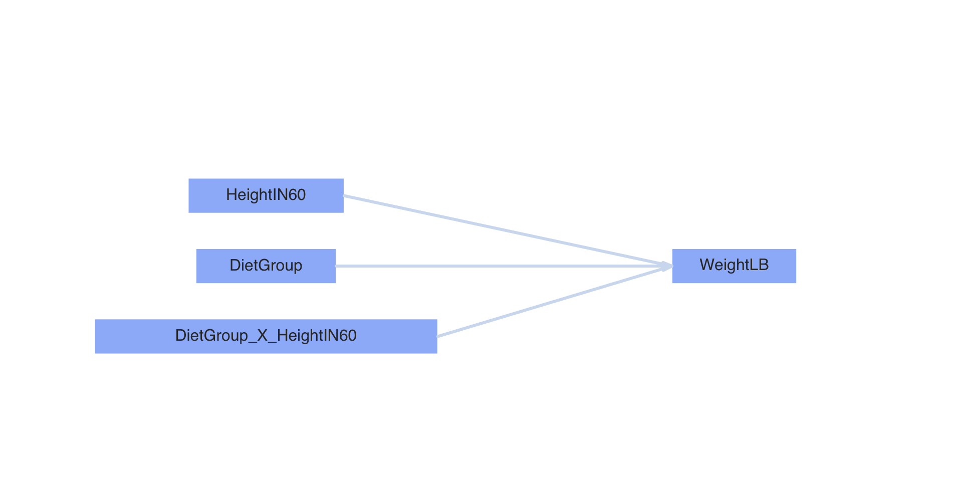
Path Diagram of Model

Linear Models with Matrices

Model (predictor) matrix:

\[\textbf{X} = \left[ \begin{array}{cccccc} 1 & -4 & 0 & 0 & 0 & 0 \\ & & \vdots & & & \\ 1 & 12 & 0 & 1 & 0 & 12 \\ \end{array} \right] \]

Coefficients vector:

\(\boldsymbol{\beta} = \left[ \begin{array}{c} \beta_0 \\ \beta_1 \\ \beta_2 \\ \beta_3 \\ \beta_4 \\ \beta_5 \\ \end{array} \right]\)

head(model.matrix(FullModelFormula, data = DietData))

  (Intercept) Height60IN factor(DietGroup)2 factor(DietGroup)3
1           1         -4                  0                  0
2           1          0                  0                  0
3           1          4                  0                  0
4           1          8                  0                  0
5           1         12                  0                  0
6           1         -6                  0                  0
  Height60IN:factor(DietGroup)2 Height60IN:factor(DietGroup)3
1                             0                             0
2                             0                             0
3                             0                             0
4                             0                             0
5                             0                             0
6                             0                             0

Linear Models with Matrices

Using matrices, we can rewrite our regression equation from

\[\text{WeightLB}_p = \beta_0 + \beta_1\text{HeightIN}_p + \beta_2 \text{Group2}_p + \beta_3 \text{Group3}_p + \beta_4\text{HeightIN}_p\text{Group2}_p + \] \[\beta_5\text{HeightIN}_p\text{Group3}_p + e_p\]

To:

\[\textbf{WeightLB} = \textbf{X}\boldsymbol{\beta} + \textbf{e}\]

Where:

• \(\textbf{WeightLB}\) is the vector of outcomes (size \(N \times 1\))
• \(\textbf{X}\) is the model (predictor) matrix (size \(N \times P\) for \(P-1\) predictors)
• \(\boldsymbol{\beta}\) is the coefficents vector (size \(P \times 1\))
• \(\textbf{e}\) is the vector of residuals (size \(N \times 1\))

Example: Predicted Values

P=6
beta = matrix(data = runif(n = 6, min = 0, max = 10), nrow = P, ncol = 1)
X = model.matrix(FullModelFormula, data=DietData)
X %*% beta # R uses %*% for matrix products

          [,1]
1    3.5041870
2    4.2407897
3    4.9773925
4    5.7139952
5    6.4505980
6    3.1358856
7    4.6090911
8    5.1615432
9    5.1615432
10   6.0822966
11  -1.5318296
12   5.4390386
13  12.4099067
14  19.3807748
15  26.3516430
16  -5.0172636
17   8.9244726
18  14.1526237
19  14.1526237
20  22.8662089
21 -25.4129828
22  -5.4996766
23  14.4136295
24  34.3269356
25  54.2402417
26 -35.3696358
27  -0.5213501
28  24.3702826
29  29.3486091
30  64.1968948

Syntax Changes: Data Section

Old Syntax Without Matrices

data {
  int<lower=0> N;
  vector[N] weightLB;
  vector[N] height60IN;
  vector[N] group2;
  vector[N] group3;
  vector[N] heightXgroup2;
  vector[N] heightXgroup3;
}

New Syntax With Matrices

data {
  int<lower=0> N;         // number of observations
  int<lower=0> P;         // number of predictors (plus column for intercept)
  matrix[N, P] X;         // model.matrix() from R 
  vector[N] y;            // outcome
  
  vector[P] meanBeta;       // prior mean vector for coefficients
  matrix[P, P] covBeta; // prior covariance matrix for coefficients
  
  real sigmaRate;         // prior rate parameter for residual standard deviation
}

Syntax Changes: Parameters Section

Old Syntax Without Matrices

parameters {
  real beta0;
  real betaHeight;
  real betaGroup2;
  real betaGroup3;
  real betaHxG2;
  real betaHxG3;
  real<lower=0> sigma;
}

New Syntax With Matrices

parameters {
  vector[P] beta;         // vector of coefficients for Beta
  real<lower=0> sigma;    // residual standard deviation
}

Defining Prior Distributions

Previously, we defined a normal prior distribution for each regression coefficient

• Univariate priors – univariate normal distribution
• Each parameter had a prior that was independent of the other parameters

When combining all parameters into a vector, a natural extension is a multivariate normal distribution

• https://en.wikipedia.org/wiki/Multivariate_normal_distribution
• Mean vector (meanBeta; size \(P \times 1\))
  • Put all prior means for these coefficients into a vector from R
• Covariance matrix (covBeta; size \(P \times P\))
  • Put all prior variances (prior \(SD^2\)) into the diagonal
  • With zeros for off diagonal, the MVN prior is equivalent to the set of independent univariate normal priors

Syntax Changes: Model Section

Old Syntax Without Matrices

model {
  beta0 ~ normal(0,1);
  betaHeight ~ normal(0,1);
  betaGroup2 ~ normal(0,1);
  betaGroup3 ~ normal(0,1);
  betaHxG2 ~ normal(0,1);
  betaHxG3 ~ normal(0,1);
  
  sigma ~ exponential(.1); // prior for sigma
  weightLB ~ normal(
    beta0 + betaHeight * height60IN + betaGroup2 * group2 + 
    betaGroup3 * group3 + betaHxG2 *heightXgroup2 +
    betaHxG3 * heightXgroup3, sigma);
}

New Syntax With Matrices

model {
  beta ~ multi_normal(meanBeta, covBeta); // prior for coefficients
  sigma ~ exponential(sigmaRate);         // prior for sigma
  y ~ normal(X*beta, sigma);              // linear model
}

See: Example Syntax in R File

Summary of Changes

• With matrices, there is less syntax to write
  • Model is equivalent
• Output, however, is not labeled with respect to parameters
  • May have to label output

# A tibble: 8 × 10
  variable    mean  median    sd   mad     q5     q95  rhat ess_bulk ess_tail
  <chr>      <dbl>   <dbl> <dbl> <dbl>  <dbl>   <dbl> <dbl>    <dbl>    <dbl>
1 lp__     -78.0   -77.7   2.09  1.93  -82.0  -75.3    1.00    2840.    4327.
2 beta[1]  147.    147.    3.17  3.09  142.   152.     1.00    3044.    4196.
3 beta[2]   -0.349  -0.352 0.485 0.475  -1.15   0.455  1.00    3258.    4432.
4 beta[3]  -24.0   -24.0   4.46  4.40  -31.3  -16.6    1.00    3340.    4801.
5 beta[4]   81.5    81.5   4.22  4.14   74.6   88.5    1.00    3438.    4785.
6 beta[5]    2.45    2.45  0.683 0.680   1.33   3.54   1.00    3579.    4813.
7 beta[6]    3.53    3.53  0.640 0.630   2.48   4.58   1.00    3550.    4266.
8 sigma      8.24    8.10  1.22  1.16    6.51  10.4    1.00    4444.    4860.

Computing Functions of Parameters

Computing Functions of Parameters

• Often, we need to compute some linear or non-linear function of parameters in a linear model
  • Missing effects (i.e., slope for Diet Group 2)
  • Simple slopes
  • \(R^2\)
• In non-Bayesian analyses, these are often formed with the point estimates of parameters
• For Bayesian analyses, however, we will seek to build the posterior distribution for any function of the parameters
  • This means applying the function to all posterior samples

Example: Need Slope for Diet Group 2

Recall our model:

\[\text{WeightLB}_p = \beta_0 + \beta_1\text{HeightIN}_p + \beta_2 \text{Group2}_p + \beta_3 \text{Group3}_p + \beta_4\text{HeightIN}_p\text{Group2}_p + \]

\[\beta_5\text{HeightIN}_p\text{Group3}_p + e_p\]

Here, \(\beta_1\) is the change in \(\text{WeightLB}_p\) per one-unit change in \(\text{HeightIN}_p\) for a person in Diet Group 1 (i.e. _p and \(\text{Group3}_p=0\))

Question: What is the slope for Diet Group 2?

• To answer, we need to first form the model when \(\text{Group2}_p = 1\): \[\text{WeightLB}_p = \beta_0 + \beta_1\text{HeightIN}_p + \beta_2 + \beta_4\text{HeightIN}_p + e_p\]
• Next, we rearrange terms that involve \(\text{HeightIN}_p\): \[\text{WeightLB}_p = (\beta_0 + \beta_2) + (\beta_1 + \beta_4)\text{HeightIN}_p + e_p\]
• From here, we can see the slope for Diet Group 2 is \((\beta_1 + \beta_4)\)
  • Also, the intercept for Diet Group 2 is \((\beta_0 + \beta_2)\)

Computing Slope for Diet Group 2

Our task: Create posterior distribution for Diet Group 2

• We must do so for each iteration we’ve kept from our MCMC chain
• A somewhat tedious way to do this is after using Stan

model05_Samples$summary()

# A tibble: 8 × 10
  variable    mean  median    sd   mad     q5     q95  rhat ess_bulk ess_tail
  <chr>      <dbl>   <dbl> <dbl> <dbl>  <dbl>   <dbl> <dbl>    <dbl>    <dbl>
1 lp__     -78.0   -77.7   2.09  1.93  -82.0  -75.3    1.00    2840.    4327.
2 beta[1]  147.    147.    3.17  3.09  142.   152.     1.00    3044.    4196.
3 beta[2]   -0.349  -0.352 0.485 0.475  -1.15   0.455  1.00    3258.    4432.
4 beta[3]  -24.0   -24.0   4.46  4.40  -31.3  -16.6    1.00    3340.    4801.
5 beta[4]   81.5    81.5   4.22  4.14   74.6   88.5    1.00    3438.    4785.
6 beta[5]    2.45    2.45  0.683 0.680   1.33   3.54   1.00    3579.    4813.
7 beta[6]    3.53    3.53  0.640 0.630   2.48   4.58   1.00    3550.    4266.
8 sigma      8.24    8.10  1.22  1.16    6.51  10.4    1.00    4444.    4860.

slopeG2 = model05_Samples$draws("beta[2]") + model05_Samples$draws("beta[5]")
summary(slopeG2)

# A tibble: 1 × 10
  variable  mean median    sd   mad    q5   q95  rhat ess_bulk ess_tail
  <chr>    <dbl>  <dbl> <dbl> <dbl> <dbl> <dbl> <dbl>    <dbl>    <dbl>
1 beta[2]   2.10   2.10 0.481 0.463  1.31  2.88  1.00    7569.    6251.

Computing the Slope Within Stan

Stan can compute these values for us–with the “generated quantities” section of the syntax

generated quantities{
  real slopeG2;
  slopeG2 = betaHeight + betaHxG2;
}

The generated quantities block computes values that do not affect the posterior distributions of the parameters–they are computed after the sampling from each iteration

• The values are then added to the Stan object and can be seen in the summary
  • They can also be plotted using the bayesplot package

model04b_Samples$summary()

# A tibble: 9 × 10
  variable       mean   median     sd    mad      q5      q95  rhat ess_bulk
  <chr>         <dbl>    <dbl>  <dbl>  <dbl>   <dbl>    <dbl> <dbl>    <dbl>
1 lp__       -150.    -149.     2.05   1.90  -153.   -147.     1.00    1813.
2 beta0         0.214    0.207  0.997  0.993   -1.42    1.86   1.00    4119.
3 betaHeight   12.1     12.0    3.54   3.45     6.33   17.9    1.00    2311.
4 betaGroup2  123.     123.    28.2   28.0     76.3   169.     1.00    3443.
5 betaGroup3  229.     229.    24.7   24.2    189.    269.     1.00    4005.
6 betaHxG2     -9.96    -9.93   5.50   5.30   -19.1    -1.01   1.00    2370.
7 betaHxG3     -8.93    -8.88   5.17   5.16   -17.3    -0.531  1.00    2593.
8 sigma        71.8     71.0    8.90   8.48    58.8    87.9    1.00    3471.
9 slopeG2       2.11     2.08   4.29   4.24    -4.96    9.10   1.00    3711.
# ℹ 1 more variable: ess_tail <dbl>

Computing the Slope with Matrices

To put this same method to use with our matrix syntax, we can form a contrast matrix

• Contrasts are linear combinations of parameters
  • You may have used these in R using the glht package

For us, we form a contrast matrix that is size \(C \times P\) where C are the number of contrasts

• The entries of this matrix are the values that multiply the coefficients
  • For \((\beta_1 + \beta_4)\) this would be
    • A one in the corresponding entry for \(\beta_1\)
    • A one in the corresponding entry for \(\beta_4\)
    • Zeros elsewhere
• \(\textbf{C} = \left[ \begin{array}{cccccc} 0 & 1 & 0 & 0 & 1 & 0 \\ \end{array} \right]\)

The contract matrix then multipies the coefficents vector to form the values:

\[\textbf{C} \boldsymbol{\beta}\]

Contrasts in Stan

We can change our Stan code to import a contrast matrix and use it in generated quantities:

data {
  int<lower=0> N;         // number of observations
  int<lower=0> P;         // number of predictors (plus column for intercept)
  matrix[N, P] X;         // model.matrix() from R 
  vector[N] y;            // outcome
  
  vector[P] meanBeta;     // prior mean vector for coefficients
  matrix[P, P] covBeta;   // prior covariance matrix for coefficients
  
  real sigmaRate;         // prior rate parameter for residual standard deviation
  
  int<lower=0> nContrasts; 
  matrix[nContrasts,P] contrast;   // contrast matrix for additional effects
}

The generated quantities would then become:

generated quantities {
  vector[nContrasts] contrasts;
  contrasts = contrastMatrix*beta;
}

See example syntax for a full demonstration

Computing \(R^2\)

We can use the generated quantities section to build a posterior distribution for \(R^2\)

There are several formulas for \(R^2\), we will use the following:

\[R^2 = 1 - \frac{RSS}{TSS} = 1 - \frac{\sum_{p=1}^{N}\left(y_p - \hat{y}_p\right)^2}{\sum_{p=1}^{N}\left(y_p - \bar{y}_p\right)^2}\]

Where:

• RSS is the regression sum of squares
• TSS is the total sum of squares
• \(\hat{y} = \textbf{X}\boldsymbol{\beta}\)
• \(\bar{y} = \sum_{p=1}^{N}\frac{y_p}{N}\)

Notice: RSS depends on sampled parameters–so we will use this to build our posterior distribution for \(R^2\)

Computing \(R^2\) in Stan

The generated quantities block can do everything we need to compute \(R^2\)

generated quantities {
  vector[nContrasts] heightSlopeG2;
  real rss;
  real totalrss;
    
  heightSlopeG2 = contrast*beta;
  
  { // anything in these brackets will not appear in summary
    vector[N] pred;
    pred = X*beta;
    rss = dot_self(y-pred); // dot_self is a stan function
    totalrss = dot_self(y-mean(y));
  }
  
  real R2;
  
  R2 = 1-rss/totalrss;
  
}

See the example syntax for a demonstration

Wrapping Up

Today we further added to our Bayesian toolset:

• How to make Stan use less syntax using matrices
• How to form posterior distributions for functions of parameters

We will use both of these features in psychometric models

Up Next

We have one more lecture on linear models that will introduce

• Methods for relative model comparisons
• Methods for checking the absolute fit of a model

Then all things we have discussed to this point will be used in our psychometric models