Introduction to Psychometric Models

Lecture 2

Today’s Lecture Objectives

An Framing Example
Latent traits
Our first graphical model (path diagram)
Psychometric models from generalized linear models

Class Discussion: Satisfaction with Life Scale

Take a look at the following items (as reported in McDonald, 1999): https://uiowa.qualtrics.com/jfe/form/SV_6J8Hakox1U4S7UW

Questions for discussion:

How would we analyze these data?
Do you know of any psychometric model that would work?

More Class Discussion: SWLS, Revised

Now, take a look at the following revised items (item stems reported in McDonald, 1999): https://uiowa.qualtrics.com/jfe/form/SV_e8rqrilRNBnT8SG

Questions for discussion:

What is different about this survey?
Does this survey seem to measure the same construct as the previous survey?
How would we analyze these data?
Do you know of any psychometric model that would work?

Latent Traits: A Big-Picture View

Latent trait theory posits there are attributes of a person (typically) that are:

Unobservable (hence the term latent)
Quantifiable
Related to tasks that can be observed

Often, these attributes are often called constructs, underscoring they are constructed and do not exist, such as:

A general or specific ability (in educational contexts)
A feature of personality, such as “extroversion” (in psychological contexts)

The same psychometric models apply regardless of the measurement context (math don’t care)

The Long History of Latent Trait Theory

Latent trait theory, as we now know it, began well before most current academic disciplines
- Educational assessments (tests) have existed for centuries
  - These seek to measure latent abilities
- The study of intelligence began in the mid 1800s
  - Intelligence is also a latent trait
Methodological innovations have often spurred empirical (discipline-specific) trait development
- Early methods were limited by mathematical and statistical theory
- The invention and wide-spread use of computers made advances in psychometrics possible
- More recent statistical innovations further shape methods (i.e., computational estimation methods using Bayes)

Latent Traits are Interdisciplinary

Many varying fields use some version of latent traits
Similar (or identical) methods are often developed separately
- Item response theory in education
- Item factor analysis in psychology
Many different terms for same ideas, such as the
- Label given to the latent trait: Factor/Ability/Attribute/Construct
- Label given to those giving the data: Examinee/Subject/Participant/Respondent/Patient/Student
What this means:
- Lots of words to keep track of, but (relatively) few concepts
- We will focus on concepts (but have a lot of words)

The Best Constructs Are Built Purposefully

Latent constructs seldom occur randomly—they are defined
- The definition typically indicates:
  - What the construct means
  - What observable behaviors are likely related to the construct
    - For a lot of what we do, observable behavior means answering questions on an assessment or survey
Therefore, modern psychometric methods are built around specifying the set of observed variables to which a latent variable relates
- No need for exploratory analyses—we define our construct and seek to falsify our definition
The term I use for “relates” is “measure”
- Educational assessment items measure some type of ability

Guiding Principles

To better understand psychometric methods and theory, I recommend you envision what you would do if latent variables were not latent
- Example: Imagine if we could directly observe mathematics ability
Then, consider what we would do with that value
- Example: We could predict how students would perform on items using logistic regression
Psychometric models essentially do this—use observed variable methods as if we know the value of the latent variable
- There are some catches, though
  - We need a data collection design that allows for such methods to be used
  - We need a more formal vetting of whether or not we did a good job measuring the construct

Measurement, Formally Defined

Measurement is the quantification of some characteristic (physical or otherwise)

Consider the measurement of length (a physical construct)
- Why? We need to know where to put things
- How? We use some type of device (a ruler, yardstick, tape measure) and note the distance from the origin
- What? The distance is then quantified with some type of unit (a unit of measure)
  - Inches, centimeters, meters, yards, etc…

Measurement of Latent Constructs

How does this differ when we cannot observe the thing we are measuring—when the construct is latent?
- We still need something we can observe—item responses for example
- We need a method to map the response to a number (like the inches)
  - Strongly agree==5?
- We also need a way to aggregate all responses to a value that represents a person
  - A score or classification
- We then need a way to ensure what we just did means what we think it does
  - Methods for validation
- We also need to remember that the values we estimate for the latent variable won’t be perfectly reliable
  - Caution needed for secondary analyses

Measurement Models

A distinguishing feature of psychometric models is the second word—they are models
We often call such models “measurement models”
Measurement models are the mathematical specification that provides the link between the latent variable(s) and the observed data
The form of such models looks different across the wide classes of measurement models (e.g., factor analysis vs. item response models) but wide generalities exist
Measurement models need:
- Distributional assumptions about the data (with link functions)
- A linear or non-linear form that predicts data from the trait(s)
The key: Observed data are being predicted by latent variable(s)

Measurement Models vs. Other Measurement Techniques

Measurement models are a different way of thinking about psychometrics than what most people without psychometric training do

A lot of the world will enumerate item response scores
- e.g., correct response == 1; strongly agree == 5
The latent trait score estimate is then formed by adding the response scores together
- The “Add Stuff* Up” model
  - Please see Lesa Hoffman for a more explicit definition of Stuff
As it turns out, the naïve adding together of item scores implies a measurement model
- Called parallel items — very strict assumptions (equal variances and covariances)

Characteristics of Latent Variables

Latent variables can have different levels of measurement (in concept, not in practice)
- Interval level (as in factor analysis and item response theory) — Continuous
  - No absolute zero, but units of the quantity are equivalent across the range of values
  - Example: A person with a value of 2 is the same distance from a person with a value of 0 as is a person with a value of -2
- Ordinal level (as in diagnostic classification models)
  - Can rank order people but not determine how far apart they may be
  - Example: Students considered masters of a topic have more ability than students considered non-masters
- Nominal level (as in latent class or finite mixture models) — Categorical
  - Groups/classes/clusters of people
  - No scale provided at all

Most Common: Continuous Latents

For most of this class, we will treat latent variables as continuous (interval level)
As they do not exist, continuous latent variables need a defined metric:
- What is their mean?
- What is their standard deviation?
Defining the metric is the first step in a latent variable model
- Called scale identification
The metric is arbitrary
- Can set differing means/variances but still have same model
- Linear transformations of parameters based on scale mean and standard deviation

Measurement Model Path Diagrams

Measurement models are often depicted in graphical format, using what is called a path diagram

Typically, latent variables are represented as objects that are circles/ovals
Using graph theory terms, a variable in a path diagram (latent or observed) is called a node
Lines connecting the variables are called edges

Latent Variable Only

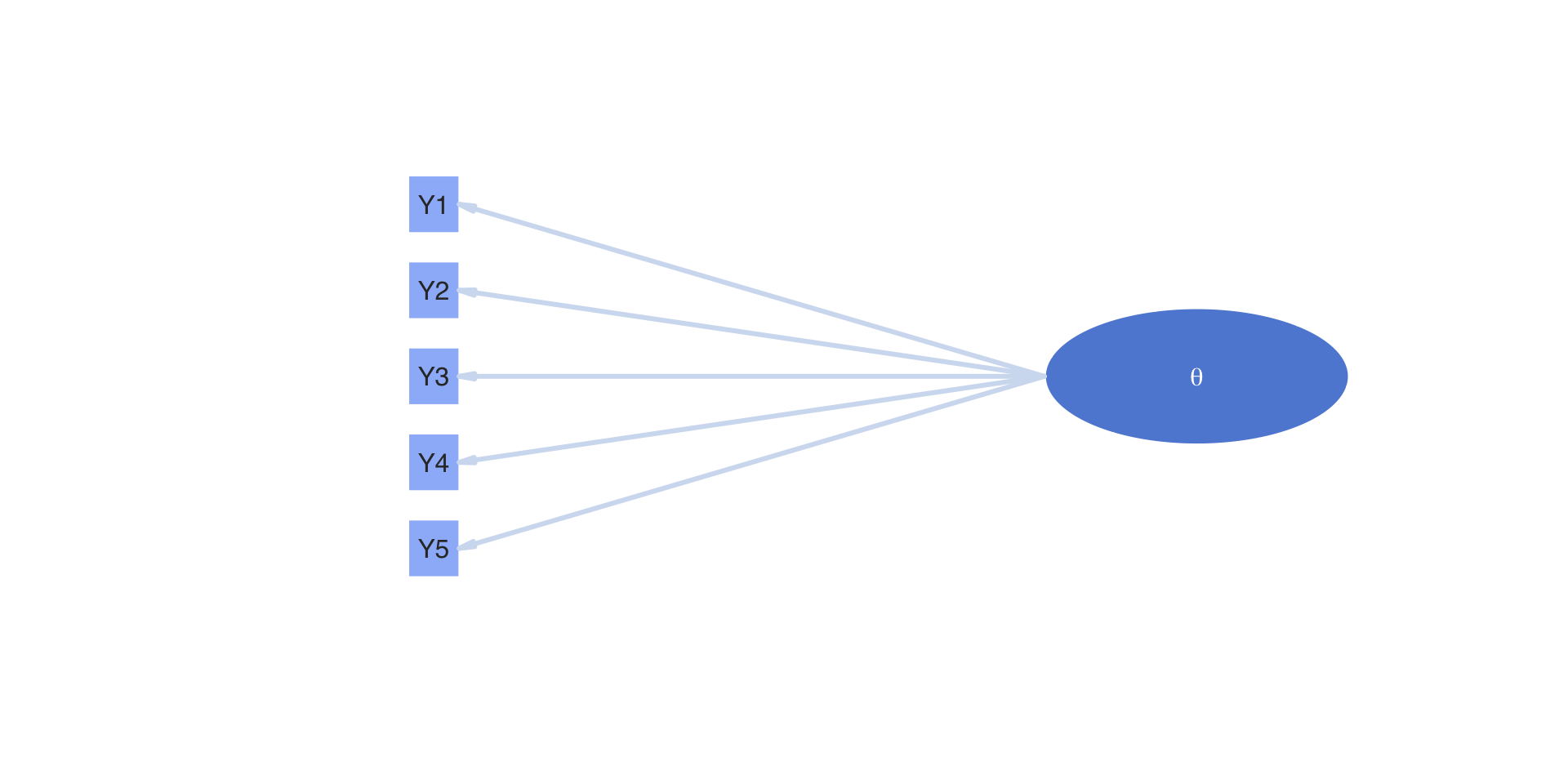
Adding Observed Variables

Measurement model path diagrams often denote observed variables with boxes

On the next slide:

The term “latent variable” is replaced with \(\theta\)
The observed variables are denoted as \(Y1\) through \(Y5\)
- Imagine these represent the five items of the scale we started class with

Path Diagram with Observed and Latent Variables

Path Diagrams: Not Models

Path diagrams are useful for depicting a measurement model but are not models

All model parameters cannot be included in the diagram
No indication about the distribution of the variables (especially needed in Bayesian psychometric modeling)

Translating a Path Diagram to a Model

Going back to our the point from before—let’s imagine the latent variable as an observed variable

An arrow (edge) indicates one variable predicts another
- The predictor is the variable on the side of the arrow without the point
- The outcome is the variable on the side of the point
If we assume the items were continuous (like linear regression), the diagram indicates a regression model for each outcome

\[ \begin{array}{c} Y_{p1} = \beta_{Y_1, 0} + \beta_{Y_1,1} \theta_p + e_{p, Y_1} \\ \end{array} \]

Interpreting the Parameters

All five regression lines implied by the model are then:

\[ \begin{array}{c} Y_{p1} = \beta_{Y_1, 0} + \beta_{Y_1,1} \theta_p + e_{p, Y_1} \\ Y_{p1} = \beta_{Y_2, 0} + \beta_{Y_2,1} \theta_p + e_{p, Y_2} \\ Y_{p3} = \beta_{Y_3, 0} + \beta_{Y_3,1} \theta_p + e_{p, Y_3} \\ Y_{p4} = \beta_{Y_4, 0} + \beta_{Y_4,1} \theta_p + e_{p, Y_4} \\ Y_{p5} = \beta_{Y_5, 0} + \beta_{Y_5,1} \theta_p + e_{p, Y_5} \\ \end{array} \]

Here:

\(\beta_{Y_i, 0}\) is the intercept of the regression line predicting the score from item \(Y_i\)
- The expected resposne score for a person who has \(\theta_p=0\)
\(\beta_{Y_i, 1}\) is the slope of the regression line predicting the score from item \(Y_i\)
- The expected change in the response score for a one-unit change in \(\theta_p\)

More Interpreting the Parameters

Also:

\(e_{p, Y_i}\) is the residual (error), indicating the difference in the predicted score for person \(p\) to item \(i\)
- Like in regression, we additionally assume:
  - \(e_{p,Y_i} \sim N\left(0, \sigma^2_{e_{Y_i}} \right)\): is normally distributed with mean zero and…
\(\sigma^2_{e_{Y_i}}\) is the residual variance of item \(Y_i\), indicating the square of how far off the prediction is on average

The five regression models are estimated simultaneously:

If \(\theta_p\) were observed, we would call this a multivariate regression
- Multivariate regression: Multiple continuous outcomes predicted by one or more predictors

More About Regression

\[Y_{pi} = \beta_{Y_i, 0} + \beta_{Y_i,1} \theta_p + e_{p, Y_i} \]

In the regression model for a single variable, what distribution do we assume about the outcome?

As error is normally distributed, the outcome takes a normal distribution \(Y_{pi} \sim N( ?, ?)\)
As \(\beta_{Y_i, 0}\), \(\beta_{Y_i,1}\), and \(\theta_p\) are constants, they move the mean of the outcome to \(\beta_{Y_i, 0} + \beta_{Y_i,1} \theta_p\)
- \(Y_{pi} \sim N( \beta_{Y_i, 0} + \beta_{Y_i,1} \theta_p, ?)\)
As error has a variance of \(\sigma^2_{e_{Y_i}}\), the outcome is assumed to have variance \(\sigma^2_{e_{Y_i}}\)
- \(Y_{pi} \sim N( \beta_{Y_i, 0} + \beta_{Y_i,1} \theta_p, \sigma^2_{e_{Y_i}})\)
Therefore, we say \(Y_{pi}\) follows a conditionally normal distribution

The Univariate Normal (Gaussian) Distribution

When we say \(Y \sim N( \mu, \sigma^2)\), that implies a probability density function (pdf).
For the univariate normal (sometimes called Gaussian) distribution, the pdf is: \[f\left(Y\right) = \frac{1}{\sqrt{2 \pi \sigma^2 }}\exp\left[\frac{\left(Y - \mu \right)^2}{2\sigma^2} \right]\]
Here, \(\pi\) is the constant 3.14 and \(\exp\) is Euler’s constant (2.71)
Of note here is that there are three components that go into the function:
- The data \(Y\)
- The mean \(\mu\) — this can be the conditional mean we had on the previous slide (formed by parameters)
- The variance \(\sigma^2\)
The key to using Bayesian methods is to know the distributions for each of the variables in the model

From Regression to CFA

When \(\theta_i\) is latent, the five-variable model becomes a confirmatory factor analysis (CFA) model

CFA: Prediction of continuous items using linear regression with one or more continuous latent variables as predictors
- The interpretations of the regression parameters are identical between linear regression and CFA

Regression and CFA Differences

The differences between CFA and regression are:

\(\theta_p\) is not observed in CFA but is observed in regression
- Therefore, we must set its mean and variance
  - There are multiple was to do this (standardized factor, marker item, etc…)—stay tuned
Each of the model parameters has a different name (and symbol denoting it) in CFA
- \(\beta_{Y_i, 0} = \mu_i\) is the item intercept
- \(\beta_{Y_i,1} = \lambda_i\) is the factor loading for an item
- \(\sigma^2_{e_{Y_i}} = \psi^2_i\) is the unique variance for an item
We must have a sufficient number of observed variables to empirically identify the latent trait

Changing Notation

Our five-item CFA model with CFA-notation:

\[ \begin{array}{c} Y_{p1} = \mu_1 + \lambda_1 \theta_p + e_{p, Y_1} \\ Y_{p2} = \mu_2 + \lambda_2 \theta_p + e_{p, Y_2} \\ Y_{p3} = \mu_3 + \lambda_3 \theta_p + e_{p, Y_3} \\ Y_{p4} = \mu_4 + \lambda_4 \theta_p + e_{p, Y_4} \\ Y_{p5} = \mu_5 + \lambda_5 \theta_p + e_{p, Y_5} \\ \end{array} \]

Measurement Models for Different Item Types

The CFA model assumes (1) continuous latent variables and (2) continuous item scores
- What should we do if we have binary items (e.g., yes/no, correct/incorrect)?
If we had observed \(\theta_p\) and wanted to predict \(Y_{1p} \in \{0,1\}\) (read as \(Y_{p1}\) takes values of either zero or one) what type of analysis would we use?
Logistic regression:

\[P\left(Y_{p1} = 1\right) = \frac{\exp \left( \beta_{Y_1,0} + \beta_{Y_1,1} \theta_p\right)}{1+\exp \left( \beta_{Y_1,0} + \beta_{Y_1,1} \theta_p\right)}\]
Alternatively: \[Logit \left( P\left(Y_{p1} = 1\right) \right) = \beta_{Y_1,0} + \beta_{Y_1,1} \theta_p\]

Interpreting of Model Parameters

\[Logit \left( P\left(Y_{p1} = 1\right) \right) = \beta_{Y_1,0} + \beta_{Y_1,1} \theta_p\]

Here:

\(\beta_{Y_1,0}\) is the intercept — the expected log odds of a correct response when \(\theta_p = 0\)
\(\beta_{Y_1,1}\) is the slope — the expected change in log odds of a correct response for a one-unit change in \(\theta_p\)
Note: there is no error variacne term…why?

Bernoulli Distributions

Using logistic regression for binary outcomes makes the assumption that the outcome follows a (conditional) Bernoulli distribution, or \(Y \sim B(p_Y)\)
- The parameter \(p_Y\) is the probability that Y equals one, or \(P\left(Y = 1\right)\)
The Bernoulli pdf (sometimes called the probability mass function as the variable is discrete) is: \[f(Y) = \left(p_Y\right)^Y \left(1-p_y \right)^{1-Y}\]
So, there is no error variance parameter in logistic regression as there is no parameter in the distribution that represents error.
- Error is represented by how far off a probability is from either zero or one

Logistic Regression with Latent Variable(s)

Back to our running example, if we had binary items and wished to form a (unidimensional) latent variable model, we would have something that looked like:

\[P\left(Y_{pi} = 1 \mid \theta_p \right) = \frac{\exp \left( \mu_i + \lambda_i \theta_p\right)}{1+\exp \left( mu_i + \lambda_i \theta_p\right)}\]

Here, the parameters retain their names from CFA:
- \(\beta_{Y_i, 0} = \mu_i\) is the item intercept
- \(\beta_{Y_i,1} = \lambda_i\) is the factor loading for an item
We call this slope-intercept parameterization
This parameterization is called item factor analysis(IFA)

From IFA to IRT

IFA and IRT are equivalent models—their parameters are transformations of each other:

\[ \begin{array}{c} a_i = \lambda_i \\ b_i = -\frac{\mu_i}{\lambda_i} \end{array} \]

This yields the discrimination-difficulty parameterization that is common in unidimensional IRT models:

\[P\left(Y_{pi} = 1 \mid \theta_p \right) = \frac{\exp \left( a_i\left( \theta_p -b_i\right)\right)}{1+\exp \left(a_i\left( \theta_p -b_i\right)\right)}\]

\(b_i\) is the item difficulty—the point on the \(\theta\) scale at which a person has a 50% chance of answering with a one
\(a_i\) is the item discrimination—the slope of a line tangent to the curve at the item difficulty
IRT models have a number of different forms of this equation (this is the two-parameter logistic 2PL model)

Generalized Linear (Psychometric) Models

A key to understanding the varying types of psychometric models is that they must map the theory (the right-hand side of the equation—\(\theta_p\)) to the type of observed data
Today we’ve seen two types of data: continuous (with a normal distribution) and binary (with a Bernoulli distribution)
For each, the right-hand side of the item model was the same
For the normal distribution:
- We had an error term but did not transform the right-hand side
For the Bernoulli distribution:
- No error term and a function used to transform the right-hand side so that the conditional mean ranged between zero and one
We will use these features in each of our models as we continue in this class
- This is also an introduction to generalized linear models

Wrapping Up

This lecture was a quick introduction to psychometric models
Latent trait theory guides the construction of items
Psychometric models then implement and test the theory
The family of model used is determined by the type of observable data