Bayesian Model Fit and Comparisons

Lecture 3c

Today’s Lecture Objectives

1. Bayesian methods for determining how well a model fits the data (absolute fit: Posterior Predictive Model Checks)
2. Bayesian methods for determining which model fits better (relative model fit: Widely Available Information Criterion and Leave One Out methods)

Absolute Model Fit: PPMC

Posterior predictive model checking (PPMC) is a Bayesian method for determining if a model fits the data

• Absolute model fit: “Does my model fit my data well?”
• Overall idea: If a model fits the data well, then simulated data based on the model will resemble the observed data
• Ingredients in PPMC:
  • Original data
    • Typically characterized by some set of statistics (i.e, sample mean, standard deviation, covariance) applied to data
  • Data simulated from posterior draws in the Markov Chain
    • Summarized by the same set of statistics

PPMC Example: Linear Models

Recall our linear model example with the Diet Data:

\[\text{WeightLB}_p = \beta_0 + \beta_1\text{HeightIN}_p + \beta_2 \text{Group2}_p + \beta_3 \text{Group3}_p + \beta_4\text{HeightIN}_p\text{Group2}_p + \]

\[\beta_5\text{HeightIN}_p\text{Group3}_p + e_p\]

We last used matrices to estimate this model, with the following results:

model06_Samples$summary(variables = c("beta", "sigma"))

# A tibble: 7 × 10
  variable    mean  median    sd   mad     q5     q95  rhat ess_bulk ess_tail
  <chr>      <dbl>   <dbl> <dbl> <dbl>  <dbl>   <dbl> <dbl>    <dbl>    <dbl>
1 beta[1]  147.    147.    3.12  3.09  142.   152.     1.00    2961.    4081.
2 beta[2]   -0.293  -0.294 0.481 0.465  -1.08   0.497  1.00    3222.    4690.
3 beta[3]  -23.1   -23.1   4.36  4.35  -30.2  -16.0    1.00    3268.    4369.
4 beta[4]   81.5    81.5   4.20  4.14   74.7   88.4    1.00    3475.    4302.
5 beta[5]    2.37    2.37  0.690 0.671   1.23   3.50   1.00    3541.    4845.
6 beta[6]    3.52    3.52  0.644 0.628   2.46   4.57   1.00    3767.    4432.
7 sigma      8.27    8.15  1.26  1.21    6.45  10.6    1.00    4323.    4850.

PPMC Process

The PPMC process is as follows

1. Select parameters from a single (sampling) iteration of the Markov chain
2. Using the selected parameters and the model, simulate a data set with the same size (number of observations/variables)
3. From the simulated data set, calculate selected summary statistics (e.g. mean)
4. Repeat steps 1-3 for a fixed number of iterations (perhaps across the whole chain)
5. When done, compare position of observed summary statistics to that of the distribution of summary statitsics from simulated data sets (predictive distribution)

Example PPMC

For our model, we have one observed variable that is in the model (\(Y_p\))

• Note, the observations in \(\textbf{X}\) are not modeled, so we do not examine these

First, let’s assemble the posterior draws:

# here, we use format = "draws_matrix" to remove the draws from the array format they default to
posteriorSample = model06_Samples$draws(variables = c("beta", "sigma"), format = "draws_matrix")
posteriorSample

# A draws_matrix: 2000 iterations, 4 chains, and 7 variables
    variable
draw beta[1] beta[2] beta[3] beta[4] beta[5] beta[6] sigma
  1      146   0.353     -27      79    2.43     2.2   9.3
  2      149   0.142     -33      79    2.06     2.4  10.5
  3      149   0.109     -27      80    2.35     3.0   8.5
  4      150   0.153     -21      80    1.72     3.0  10.5
  5      140  -0.031     -17      86    1.99     3.1   9.3
  6      141   0.307     -19      89    2.46     2.5   9.2
  7      149   0.590     -23      79    0.66     2.9   8.0
  8      146  -0.362     -22      82    3.02     3.4   7.3
  9      146  -0.238     -25      84    2.05     3.6   6.6
  10     145  -0.809     -20      81    3.07     3.7   6.7
# ... with 7990 more draws

Example PPMC

Next, we take one draw at random:

sampleIteration = sample(x = 1:nrow(posteriorSample), size = 1, replace = TRUE)
sampleIteration

[1] 3120

posteriorSample[sampleIteration, ]

# A draws_matrix: 1 iterations, 1 chains, and 7 variables
      variable
draw   beta[1] beta[2] beta[3] beta[4] beta[5] beta[6] sigma
  3120     148   -0.26     -27      79     2.9     3.6   6.4

Example PPMC

We then generate data based on this sampled iteration and our model distributional assumptions:

betaVector = matrix(data = posteriorSample[sampleIteration, 1:6], ncol = 1)
betaVector

           [,1]
[1,] 148.273000
[2,]  -0.263068
[3,] -27.127900
[4,]  78.629600
[5,]   2.867040
[6,]   3.578690

sigma = posteriorSample[sampleIteration, 7]

conditionalMeans = model06_predictorMatrix %*% betaVector

simData = rnorm(n = N, mean = conditionalMeans, sd = sigma)

Next, let’s take the mean and standard deviation of the simulated data:

simMean = mean(simData)
simMean

[1] 170.3747

simSD = sd(simData)
simSD

[1] 49.91996

Looping Across All Posterior Samples

We then repeat this process for a set number of samples (here, we’ll use each posterior draw)

simMean = rep(NA, nrow(posteriorSample))
simSD = rep(NA, nrow(posteriorSample))
for (iteration in 1:nrow(posteriorSample)){
  betaVector = matrix(data = posteriorSample[iteration, 1:6], ncol = 1)
  sigma = posteriorSample[iteration, 7]

  conditionalMeans = model06_predictorMatrix %*% betaVector

  simData = rnorm(n = N, mean = conditionalMeans, sd = sigma)
  simMean[iteration] = mean(simData)
  simSD[iteration] = sd(simData)
}
par(mfrow = c(1,2))
hist(simMean)
hist(simSD)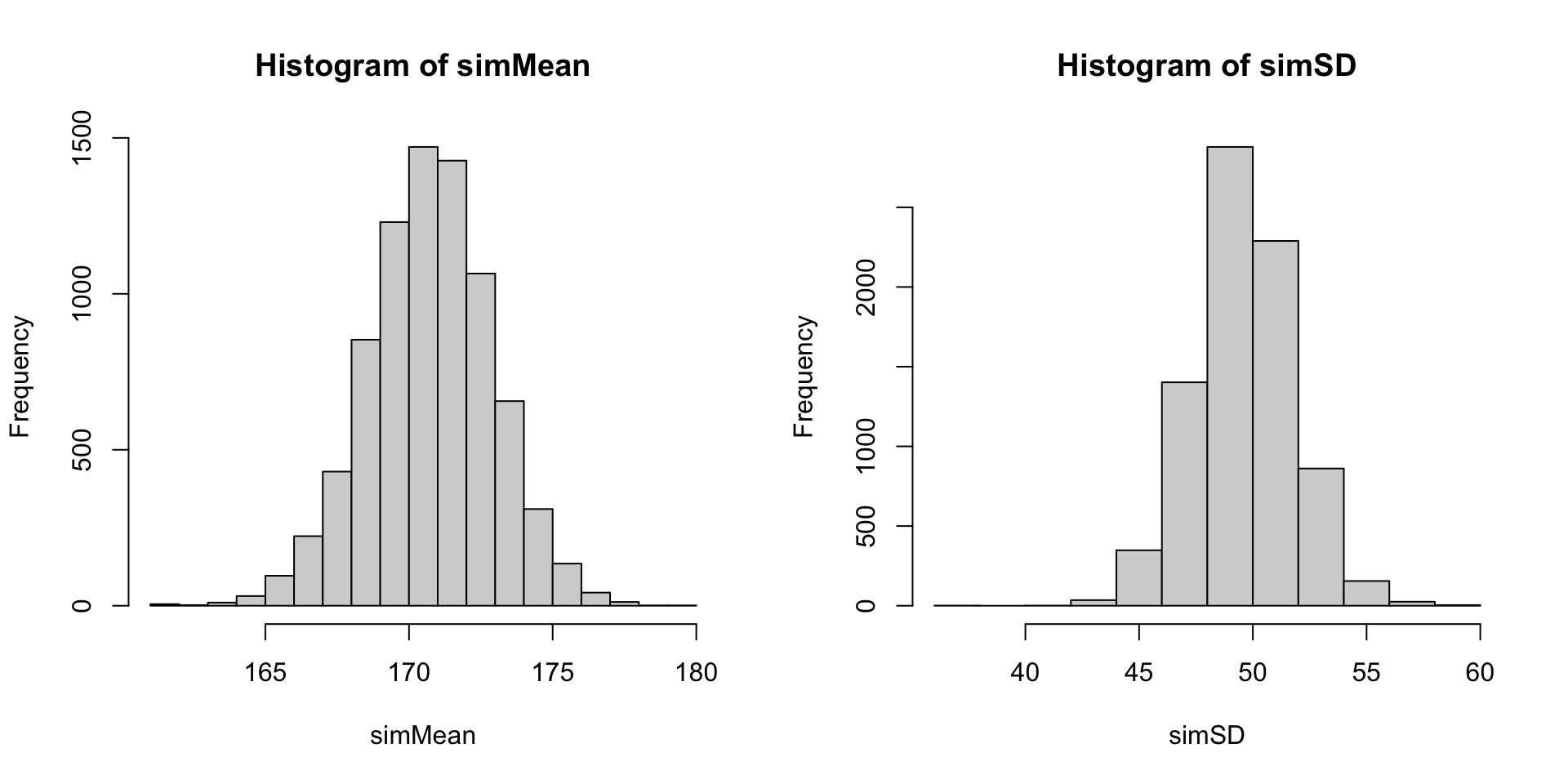

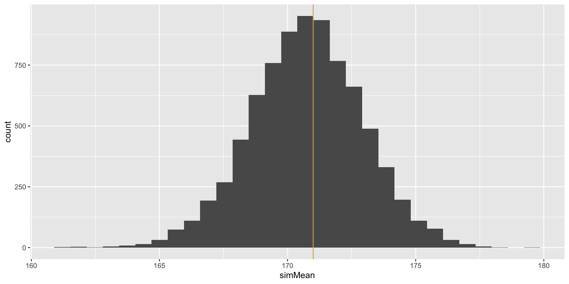
##Comparison with Observed Mean

We can now compare our observed mean and standard deviation with that of the sampled values

ggplotData = data.frame(simMean = simMean, simSD = simSD)
ggplot(data = ggplotData, aes(x = simMean)) + geom_histogram() + geom_vline(xintercept = mean(DietData$WeightLB), color = "orange")

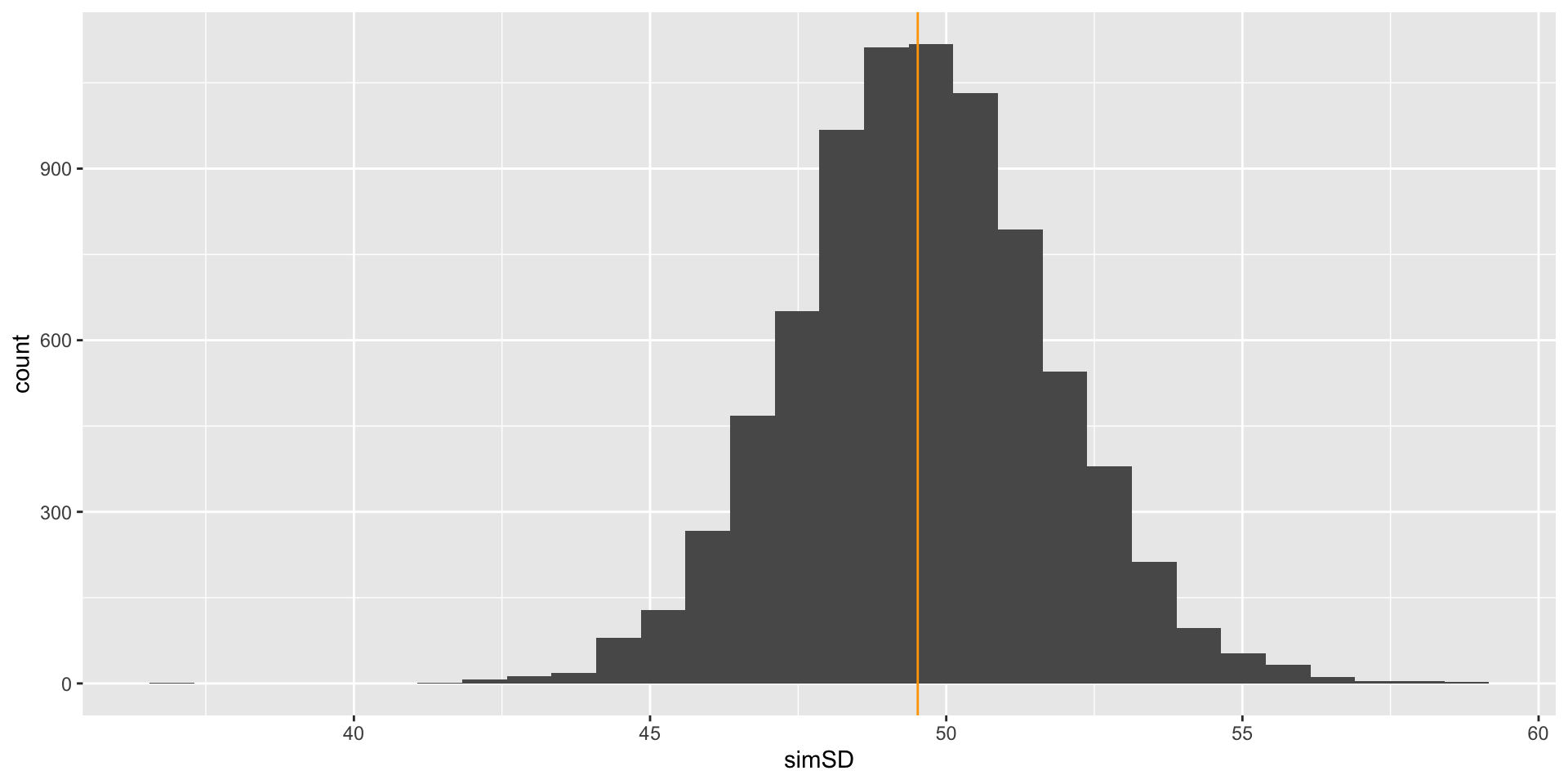
Comparison with Observed SD

We can now compare our observed mean and standard deviation with that of the sampled values

ggplot(data = ggplotData, aes(x = simSD)) + geom_histogram() + geom_vline(xintercept = sd(DietData$WeightLB), color = "orange")

PPMC Charactaristics

PPMC methods are very useful

• They provide a visual way to determine if the model fits the observed data
• They are the main method of assessing absolute fit in Bayesian models
• Absolute fit assesses if a model fits the data

But, there are some drawbacks to PPMC methods

• Almost any statistic can be used
  • Some are better than others
• No standard determining how much misfit is too much
• May be overwhelming to compute depending on your model

Posterior Predictive P-Values

We can quantify misfit from PPMC using a type of “p-value”

• The Posterior Predictive P-Value: The proportion of times the statistic from the simulated data exceeds that of the real data
• Useful to determine how far off a statistic is from its posterior predictive distribution

For the mean:

# PPP-value for mean
length(which(simMean > mean(DietData$WeightLB)))/length(simMean)

[1] 0.456125

For the standard deviation:

# PPP-value for mean
length(which(simSD > sd(DietData$WeightLB)))/length(simSD)

[1] 0.506625

If these p-values were either (a) near zero or (b) near one then this indicates how far off your data are from their predictive distribution

See the example file for comparing between two sets of priors

PPMC and PPP in Stan

We can use the generated quantities section of Stan syntax to compute these for us:

generated quantities{

  // general quantities used below:
  vector[N] y_pred;
  y_pred = X*beta; // predicted value (conditional mean)

  // posterior predictive model checking
  array[N] real y_rep;
  y_rep = normal_rng(y_pred, sigma);
  
  real mean_y = mean(y);
  real sd_y = sd(y);
  real mean_y_rep = mean(to_vector(y_rep));
  real<lower=0> sd_y_rep = sd(to_vector(y_rep));
  int<lower=0, upper=1> mean_gte = (mean_y_rep >= mean_y);
  int<lower=0, upper=1> sd_gte = (sd_y_rep >= sd(y));
  
}

Which gives us:

model06_Samples$summary(variables = c("mean_y_rep", "sd_y_rep", "mean_gte", "sd_gte"))

# A tibble: 4 × 10
  variable      mean median    sd   mad    q5   q95  rhat ess_bulk ess_tail
  <chr>        <dbl>  <dbl> <dbl> <dbl> <dbl> <dbl> <dbl>    <dbl>    <dbl>
1 mean_y_rep 171.     171.  2.17   2.06 167.  174.   1.00    8737.    7374.
2 sd_y_rep    49.6     49.5 2.20   2.14  46.0  53.2  1.00    8247.    6905.
3 mean_gte     0.441    0   0.496  0      0     1    1.00    8409.      NA 
4 sd_gte       0.505    1   0.500  0      0     1    1.00    8759.      NA 

Relative Model Fit

Relative Model Fit

Relative model fit: Used to compare two (or more) competing models

• In non-Bayesian models, Information Criteria are often used to make comparisons
  • AIC, BIC, etc.
  • The model with the lowest index is the model that fits best
• Bayesian model fit is similar
  • Uses an index value
  • The model with the lowest index is the model that fits best
• Recent advances in Bayesian model fit use indices that are tied to making cross-validation predictions:
  • Fit model leaving one observation out
  • Calculate statistics related to prediction (for instance, log-likelihood of that observation conditional on model parameters)
  • Do for all observations
• Newer Bayesian indices try to mirror these leave-one-out predictions (but approximate these due to time constraints)

Bayesian Model Fit Indices

Way back when (late 1990s and early 2000s), the Deviance Information Criterion was used for relative Bayesian model fit comparisons

\[\text{DIC} = p_D + \overline{D\left(\theta\right)},\]

where the estimated number of parameters is:

\[p_D = \overline{D\left(\theta\right)} - D\left(\bar{\theta}\right), \]

and where

\[ D\left( \theta\right) = -2 \log \left(p\left(y|\theta\right)\right)+C\]

C is a constant that cancels out when model comparisons are made

Here,

• \(\overline{D\left(\theta\right)}\) is the average log likelihood of the data (\(y\)) given the parameters (\(\theta\)) computed across all samples
• \(D\left(\bar{\theta}\right)\) is the log likelihood of the data (\(y\)) computed at the average of the parameters (\(\bar{\theta}\)) computed across all samples

Newer Methods

The DIC has fallen out of favor recently

• Has issues when parameters are discrete
• Not fully Bayesian (point estimate of average of parameter values)
• Can give negative values for estimated numbers of parameters in a model

WAIC (Widely applicable or Watanabe-Akaike information criterion, Watanabe, 2010) corrects some of the problems with DIC:

• Fully Bayesian (uses entire posterior distribution)
• Asymptotically equal to Bayesian cross-validation
• Invariant to parameterization

LOO: Leave One Out via Pareto Smoothed Importance Sampling

More recently, approximations to LOO have gained popularity

• LOO via Pareto Smoothed Importance Sampling attempts to approximate the process of leave-one-out cross-validation using a sampling based-approach
  • Gives a finite-sample approximation
  • Implemented in Stan
  • Can quickly compare models
  • Gives warnings when it may be less reliable to use
• The details are very technical, but are nicely compiled in Vehtari, Gelman, and Gabry (2017) (see preprint on arXiv at https://arxiv.org/pdf/1507.04544.pdf)
• Big picture:
  • Can compute WAIC and/or LOO via Stan’s loo package
  • LOO also gives variability for model comparisons

Model Comparisons via Stan

The core of WAIC and LOO is the log-likelihood of the data conditional on the model parameters, as calculated for each observation in the sample of the model:

• We can calculate this using the generated quantities block in Stan:

generated quantities{

  // general quantities used below:
  vector[N] y_pred;
  y_pred = X*beta; // predicted value (conditional mean)

  // WAIC and LOO for model comparison
  
  array[N] real log_lik;
  for (person in 1:N){
    log_lik[person] = normal_lpdf(y[person] | y_pred[person], sigma);
  }
}  

WAIC in Stan

• Using the loo package, we can calculate WAIC with the waic() function

waic(model06_Samples$draws("log_lik"))

Computed from 8000 by 30 log-likelihood matrix

          Estimate   SE
elpd_waic   -109.7  6.9
p_waic         6.8  2.7
waic         219.3 13.7

4 (13.3%) p_waic estimates greater than 0.4. We recommend trying loo instead. 

• Here:
  • elpd_waic is the expected log pointwise predictive density for WAIC
  • p_waic is the WAIC calculation of number of model parameters (a penalty to the likelihood for more parameters)
  • waic is the WAIC index used for model comparisons (lowest value is best fitting; -2*elpd_waic)

Note: WAIC needs a “log_lik” variable in the model analysis to be calculated correctly * That is up to you to provide!!

LOO in Stan

• Using the loo package, we can calculate the PSIS-LOO using cmdstanr objects with the $loo() function:

model06_Samples$loo()

Computed from 8000 by 30 log-likelihood matrix

         Estimate   SE
elpd_loo   -110.3  7.2
p_loo         7.5  3.1
looic       220.6 14.4
------
Monte Carlo SE of elpd_loo is NA.

Pareto k diagnostic values:
                         Count Pct.    Min. n_eff
(-Inf, 0.5]   (good)     26    86.7%   1476      
 (0.5, 0.7]   (ok)        3    10.0%   433       
   (0.7, 1]   (bad)       1     3.3%   33        
   (1, Inf)   (very bad)  0     0.0%   <NA>      
See help('pareto-k-diagnostic') for details.

Note: LOO needs a “log_lik” variable in the model analysis to be calculated correctly

• That is up to you to provide!!
• If named “log_lik” then you don’t need to provide the function an argument

Notes about LOO

model06_Samples$loo()

Computed from 8000 by 30 log-likelihood matrix

         Estimate   SE
elpd_loo   -110.3  7.2
p_loo         7.5  3.1
looic       220.6 14.4
------
Monte Carlo SE of elpd_loo is NA.

Pareto k diagnostic values:
                         Count Pct.    Min. n_eff
(-Inf, 0.5]   (good)     26    86.7%   1476      
 (0.5, 0.7]   (ok)        3    10.0%   433       
   (0.7, 1]   (bad)       1     3.3%   33        
   (1, Inf)   (very bad)  0     0.0%   <NA>      
See help('pareto-k-diagnostic') for details.

Here:

• elpd_loo is the expected log pointwise predictive density for LOO
• p_loo is the LOO calculation of number of model parameters (a penalty to the likelihood for more parameters)
• looic is the LOO index used for model comparisons (lowest value is best fitting; -2*elpd_loo)

Also, you get a warning if to many of your sampled values have bad diagnostic values

• See https://mc-stan.org/loo/articles/online-only/faq.html#high_khat

Comparing Models with WAIC

To compare models with WAIC, take the one with the lowest value:

waic(model06_Samples$draws("log_lik"))

Computed from 8000 by 30 log-likelihood matrix

          Estimate   SE
elpd_waic   -109.7  6.9
p_waic         6.8  2.7
waic         219.3 13.7

4 (13.3%) p_waic estimates greater than 0.4. We recommend trying loo instead. 

waic(model06b_Samples$draws("log_lik"))

Computed from 8000 by 30 log-likelihood matrix

          Estimate   SE
elpd_waic   -370.2 30.9
p_waic        17.2  4.1
waic         740.3 61.8

12 (40.0%) p_waic estimates greater than 0.4. We recommend trying loo instead. 

Comparing Models with LOO

To compare models with LOO, the loo package has a built-in comparison function:

# comparing two models with loo:
loo_compare(list(uniformative = model06_Samples$loo(), informative = model06b_Samples$loo()))

             elpd_diff se_diff
uniformative    0.0       0.0 
informative  -259.8      33.1 

This function calculates the standard error of the difference in ELPD between models

• The SE gives an indication of the standard error in the estimate (relative to the size)
• Can use this to downweight the choice of models when the standard error is high
• Note: elpd_diff is looic divided by -2 (on the log-likelihood scale, not the deviance scale)
  • Here, we interpret the result as the model with uninformative priors is preferred to the model with informative priors
  • The size of the elpd_diff is much larger than the standard error, indicating we can be fairly certain of this result

General Points about Bayesian Model Comparison

• Note, WAIC and LOO will converge as sample size increases (WAIC is asymptotic value of LOO)
• Latent variable models present challenges
  • Need log likelihood with latent variable integrated out
• Missing data models present challenges
  • Need log likelihood with missing data integrated out
• Generally, using LOO is recommended (but providing both is appropriate)

Wrapping Up

The three-part lecture (plus example) using linear models was built to show nearly all parts needed in a Bayesian analysis

• MCMC specifications
• Prior specifications
• Assessing MCMC convergence
• Reporting MCMC results
• Determining if a model fits the data (absolute fit)
• Determining which model fits the data better (relative fit)

All of these topics will be with us when we start psychometric models in our next lecture