Generalized Measurement Models: An Introduction

Today’s Lecture Objectives

Introduce measurement (psychometric) models in general
Describe the steps needed in a psychometric model analysis
Dive deeper into the observed-variables modeling aspect

Example Data: Conspiracy Theories

Today’s example is from a bootstrap resample of 177 undergraduate students at a large state university in the Midwest. The survey was a measure of 10 questions about their beliefs in various conspiracy theories that were being passed around the internet in the early 2010s. Additionally, gender was included in the survey. All items responses were on a 5- point Likert scale with:

Strongly Disagree
Disagree
Neither Agree or Disagree
Agree
Strongly Agree

Please note, the purpose of this survey was to study individual beliefs regarding conspiracies. The questions can provoke some strong emotions given the world we live in currently. All questions were approved by university IRB prior to their use.

Our purpose in using this instrument is to provide a context that we all may find relevant as many of these conspiracy theories are still prevalent today.

Conspiracy Theory Questions 1-5

Questions:

The U.S. invasion of Iraq was not part of a campaign to fight terrorism, but was driven by oil companies and Jews in the U.S. and Israel.
Certain U.S. government officials planned the attacks of September 11, 2001 because they wanted the United States to go to war in the Middle East.
President Barack Obama was not really born in the United States and does not have an authentic Hawaiian birth certificate.
The current financial crisis was secretly orchestrated by a small group of Wall Street bankers to extend the power of the Federal Reserve and further their control of the world’s economy.
Vapor trails left by aircraft are actually chemical agents deliberately sprayed in a clandestine program directed by government officials.

Conspiracy Theory Questions 6-10

Questions:

Billionaire George Soros is behind a hidden plot to destabilize the American government, take control of the media, and put the world under his control.
The U.S. government is mandating the switch to compact fluorescent light bulbs because such lights make people more obedient and easier to control.
Government officials are covertly Building a 12-lane "NAFTA superhighway" that runs from Mexico to Canada through America’s heartland.
Government officials purposely developed and spread drugs like crack-cocaine and diseases like AIDS in order to destroy the African American community.
God sent Hurricane Katrina to punish America for its sins.

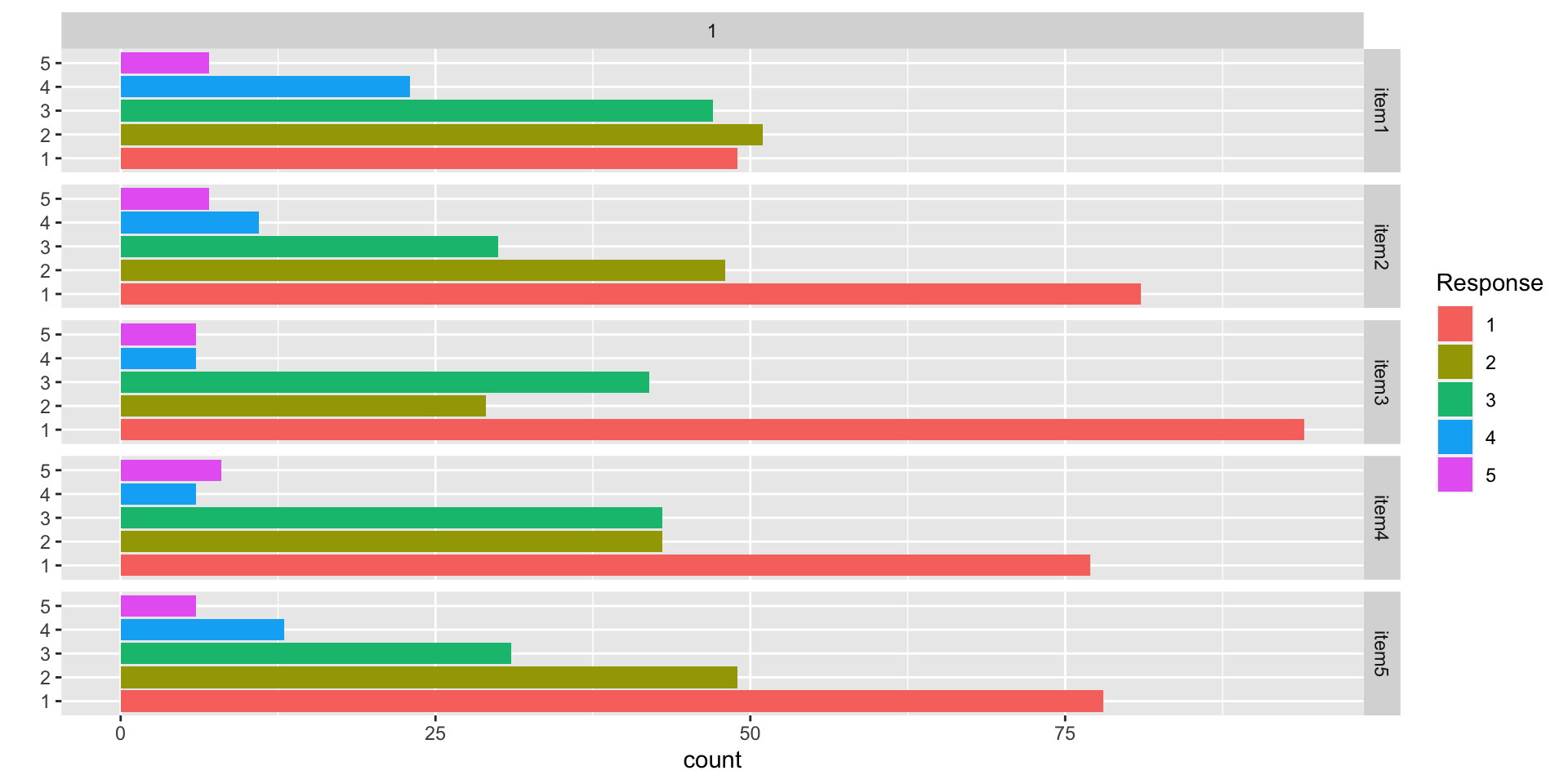
Data Visualization: Q1-Q5

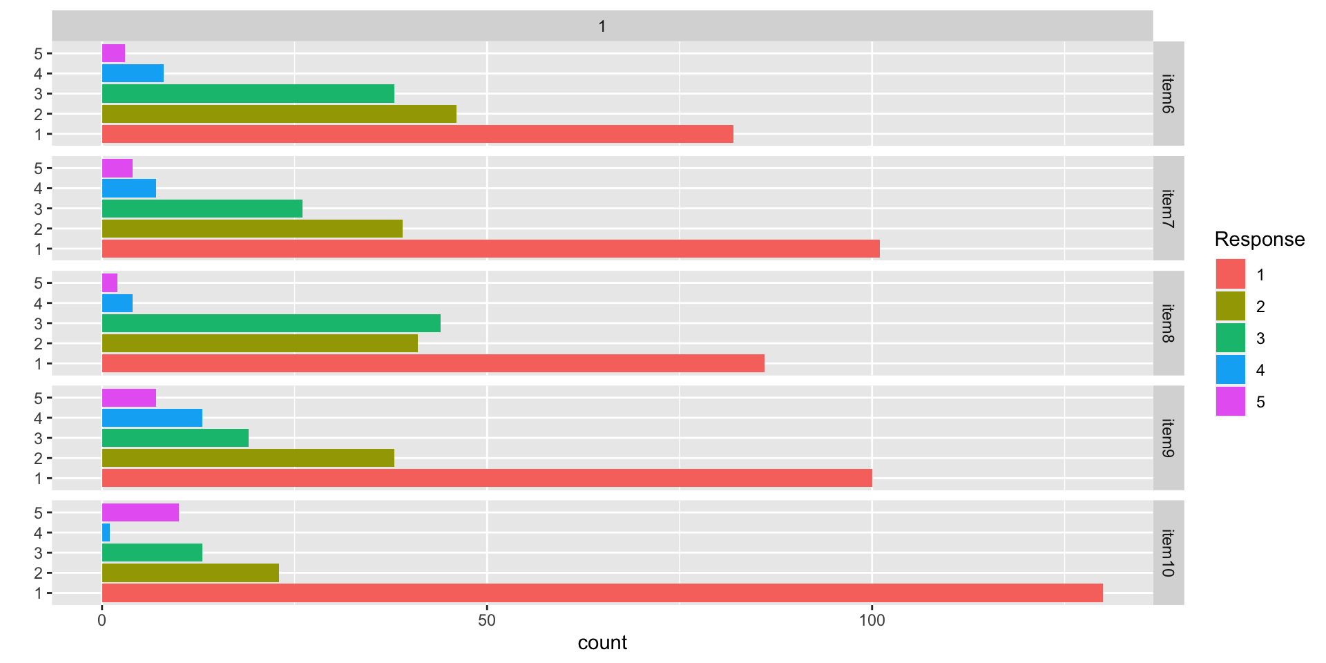
Data Visualization: Q6-Q10

Building Measurement Models

Measurement Model Analysis Steps

Specify model
Specify scale identification method for latent variables
Estimate model
Examine model-data fit
Iterate between steps 1-4 until adequate fit is achieved

Measurement Model Auxiliary Components

Score estimation (and secondary analyses with scores)
Item evaluation
Scale construction
Equating
Measurement invariance/differential item functioning

Model Specification

Recall our lecture on measurement models where we tried to describe the model itself.

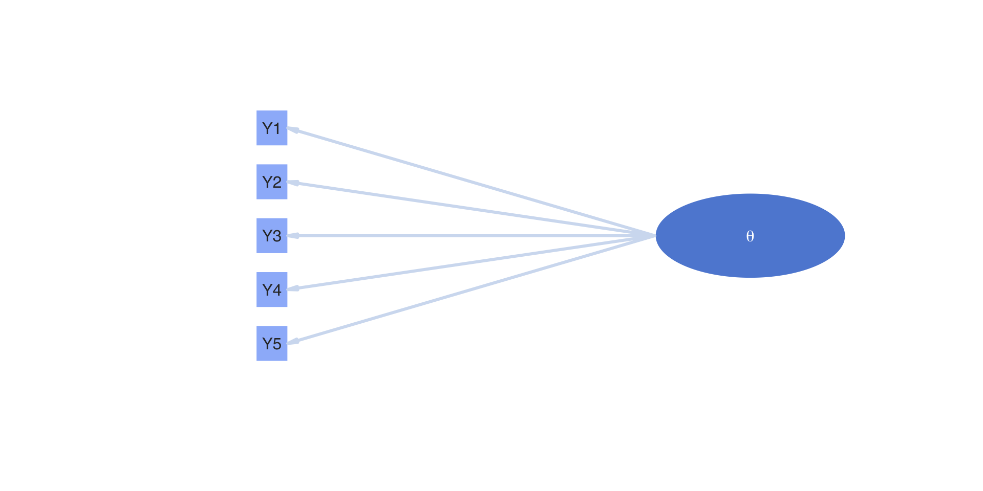
One way of doing this was through a path model:

Building a Measurement Model

The path model on the previous slide showed:

One latent variable (\(\theta\))
Five observed variables (\(Y_1\), \(Y_2\), \(Y_3\), \(Y_4\), \(Y_5\))

Each line (edge) of the path diagram implies a relationship that becomes (for one observed variable):

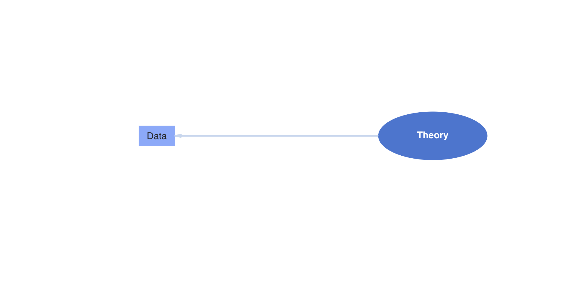
Building a Measurement Model

The Theory Side:

Latent variable(s)
Other effects as needed by a model
- Random effects (a type of latent variable)
- Testlet effects (a type of latent variable)
- Other observed variables (e.g., DIF/Measurement Invariance)

The Data Side:

Outcomes (more specifically, a function applied to one or more statistics of the outcome)
- An assumed distribution for each outcome
- A key statistic of the outcome for the model (the mean, typically)
- A link function

Example

An example for one outcome and one latent variable:

\[ f(E\left(Y_{pi} \mid \theta_p\right) ) = \mu_i + \lambda_i \theta_p \]

The right-hand side (for the latent variables) is fairly standard across models

The “theory” in my wording
In this class, all latent variables will be continuous

The left-hand side will differ by:

The “data” in my wording
Types of observed data
Additional assumptions (e.g., parameter constraints)

Latent Variables

The Latent Variables

Latent variables are built by specification:

What is their distribution? (nearly all are normally distributed)
How do you specify their scale: mean and standard deviation? (step two in our model analysis steps)

You create latent variables by specifying which items measure which latent variables in an analysis model

Called different names by different fields:
- Alignment (educational measurement)
- Factor pattern matrix (factor analysis)
- Q-matrix (Question matrix; diagnostic models and multidimensional IRT)

Alignment Task for Class

From the 10 items in our conspiracy theory example, please try to answer the following questions:

How many latent dimensions underlie these items?
Which items do you believe measure each dimension?

Note, this task should typically occur prior to writing items

Decide what you are measuring first
Then create items to measure each dimension

If an item measures a dimension, put a 1 in the column of the dimension:

       Government NonGovernment
item1           0             0
item2           0             0
item3           0             0
item4           0             0
item5           0             0
item6           0             0
item7           0             0
item8           0             0
item9           0             0
item10          0             0

From Q-matrix to Model

The alignment provides a specification of which latent variables are measured by which items

Sometimes we say items “load onto” factors

The mathematical definition of either of these terms is simply whether or not a latent variable appears as a predictor for an item

For instance, item one appears to measure government conspiracies, meaning its alignment (row vector of the Q-matrix) would be:

   Government NonGovernment 
            1             0

The model for the first item is then built with only the factors measured by the item as being present:

\[ f(E\left(Y_{p1} \mid \boldsymbol{\theta}_p\right) ) = \mu_1 + \lambda_{11} \theta_{p1} \]

From Q-matrix to Model

The model for the first item is then built with only the factors measured by the item as being present:

\[ f(E\left(Y_{p1} \mid \boldsymbol{\theta}_p\right) ) = \mu_1 + \lambda_{11} \theta_{p1} \]

Where:

\(\mu_1\) is the item intercept
\(\lambda_{11}\) is the factor loading for item 1 (the first subscript) for factor 1 (the second subscript)
\(\theta_{p1}\) is the value of the latent variable for person \(p\) and factor 1

The second factor is not included in the model for the item.

More Q-matrix Stuff

We could show the model with the Q-matrix entries:

\[ f(E\left(Y_{p1} \mid \boldsymbol{\theta}_p\right) ) = \mu_1 + q_{11}\left( \lambda_{11} \theta_{p1} \right) + q_{12}\left( \lambda_{12} \theta_{p2} \right) = \mu_1 + \boldsymbol{\lambda}_{1}^T \text{diag}\left(\boldsymbol{q}_i \right) \boldsymbol{\theta}_p \]

Where:

\[ \boldsymbol{\lambda}_{1} = \left[ \begin{array}{cc} \lambda_{11} & \lambda_{12} \end{array} \right]^T \]

\[ \text{diag}\left(\boldsymbol{q}_i \right) = \boldsymbol{q}_i \left[ \begin{array}{cc} 1 & 0 \\ 0 & 1 \end{array} \right] = \left[ \begin{array}{cc} 1 & 0 \\ \end{array} \right] \left[ \begin{array}{cc} 1 & 0 \\ 0 & 1 \end{array} \right] = \left[ \begin{array}{cc} 1 & 0 \\ 0 & 0 \end{array} \right] \]

\[ \boldsymbol{\theta}_p = \left[ \begin{array}{cc} \theta_{p1} & \theta_{p2} \\ \end{array} \right] \]

The Q-matrix functions like a partial version of the model (predictor) matrix that we saw in linear models

Multiple Item Models

Each item has its own model

\[ \begin{array}{c} f(E\left(Y_{p1} \mid \boldsymbol{\theta}_p\right) ) = \mu_1 + \lambda_{11} \theta_{p1} \\ f(E\left(Y_{p2} \mid \boldsymbol{\theta}_p\right) ) = \mu_2 + \lambda_{21} \theta_{p1} \\ f(E\left(Y_{p3} \mid \boldsymbol{\theta}_p\right) ) = \mu_3 + \lambda_{32} \theta_{p2} \\ f(E\left(Y_{p4} \mid \boldsymbol{\theta}_p\right) ) = \mu_4 + \lambda_{42} \theta_{p2} \\ f(E\left(Y_{p5} \mid \boldsymbol{\theta}_p\right) ) = \mu_5 + \lambda_{51} \theta_{p1} \\ f(E\left(Y_{p6} \mid \boldsymbol{\theta}_p\right) ) = \mu_6 + \lambda_{62} \theta_{p2} \\ f(E\left(Y_{p7} \mid \boldsymbol{\theta}_p\right) ) = \mu_7 + \lambda_{71} \theta_{p1} \\ f(E\left(Y_{p8} \mid \boldsymbol{\theta}_p\right) ) = \mu_8 + \lambda_{81} \theta_{p1} \\ f(E\left(Y_{p9} \mid \boldsymbol{\theta}_p\right) ) = \mu_9 + \lambda_{91} \theta_{p1} \\ f(E\left(Y_{p10} \mid \boldsymbol{\theta}_p\right) ) = \mu_10 + \lambda_{10,2} \theta_{p2} \\ \end{array} \]

General Forms vs. Specific Models

Up to this point, we’ve talked generally about the right-hand side of each item’s model

Some models are differentiated by constraints imposed on the right-hand side parameters
- For instance, the Rasch model (or parallel items model) constrains all loadings for a factor to be equal

In general, however, I find it easier to work with the linear model version of each item equation

Provides a good context for each item
Is (somewhat) easy to implement

Latent Variable Distributions

After building the Q-matrix, we next need to specify the distribution for each latent variable in the model

Most commonly, a normal distribution is used for each latent variable
- Model families with normally distributed latent variables:
  - Confirmatory factor analysis
  - Item response theory
  - Unfolding models
The distribution of the latent variables is the same as specifying a Bayesian prior distribution for the latent variables
If a set of latent variables is multivariate normal, then each is univariate normal

More on Latent Variable Distributions

In general, any distribution can be used. In practice, few are chosen

Not many non-normal distributions have been shown to be useful
- Care is needed as non-normal distributions can impose odd constraints that may cause bias in other parameters
Two cases of non-normal distributions that have most prevalence:
- Bernoulli (or Multivariate Bernoulli) in diagnostic models
- Multinomial (or categorical) in finite mixture models

Our Example: Multivariate Normal Distribution

For our example, we will assume the set of traits follows a multivariate normal distribution

\[ f\left(\boldsymbol{\theta}_p \right) = \left(2 \pi \right)^{-\frac{D}{2}} \det\left(\boldsymbol{\Sigma}_\theta \right)^{-\frac{1}{2}}\exp\left[-\frac{1}{2}\left(\boldsymbol{\theta}_p - \boldsymbol{\mu}_\theta \right)^T\boldsymbol{\Sigma}_\theta^{-1}\left(\boldsymbol{\theta}_p - \boldsymbol{\mu}_\theta \right) \right] \]

Where:

\(\pi \approx 3.14\)
\(D\) is the number of latent variables (dimensions)
\(\boldsymbol{\Sigma}_\theta\) is the covariance matrix of the latent variables
- \(\boldsymbol{\Sigma}_\theta^{-1}\) is the inverse of the covariance matrix
\(\boldsymbol{\mu}_\theta\) is the mean vector of the latent variables
\(\det\left( \cdot\right)\) is the matrix determinant function
\(\left(\cdot \right)^T\) is the matrix transpose operator

Alternatively, we would specify \(\boldsymbol{\theta}_p \sim N_D\left( \boldsymbol{\mu}_\theta, \boldsymbol{\Sigma}_\theta \right)\); but, we cannot always estimate \(\boldsymbol{\mu}_\theta\) and \(\boldsymbol{\Sigma}_\theta\)

Identification of Latent Traits, Part 1

Psychometric models require two types of identification to be valid:

Empirical Identification

The minimum number of items that must measure each latent variable
From CFA: three observed variables for each latent variable (or two if the latent variable is correlated with another latent variable)

Bayesian priors can help to make models with fewer items than these criteria suggest estimable

The parameter estimates (item parameters and latent variable estimates) often have MCMC convergence issues and should not be trusted
Use the CFA standard in your work

Identification of Latent Traits, Part 2

Psychometric models require two types of identification to be valid:

Scale Identification (i.e., what the mean/variance is for each latent variable)

The additional set of constraints needed to set the mean and standard deviation (variance) of the latent variables
Two main methods to set the scale:
- Marker item parameters
  - For variances: Set the loading/slope to one for one observed variable per latent variable
    - Can estimate the latent variable’s variance (the diagonal of \(\boldsymbol{\Sigma}_\theta\))
  - For means: Set the item intercept to one for one observed variable perlatent variable
    - Can estimate the latent variable’s mean (in \(\boldsymbol{\mu}_\theta\))
- Standardized factors
  - Set the variance for all latent variables to one
  - Set the mean for all latent variables to zero
  - Estimate all unique off-diagonal correlations (covariances) in \(\boldsymbol{\Sigma}_\theta\)

More on Scale Identification

Bayesian priors can let you believe you can estimate more parameters than the non-Bayesian standards suggest

For instance, all item parameters and the latent variable means/variances

Like empirical identification, these estimates are often unstable and are not recommended

Most common:

Standardized latent variables
- Used for scale development and/or when scores are of interest directly
Marker item for latent variables and zero means
- Used for cases where latent variables may become outcomes (and that variance needs explained)

Important Point: Regardless of model choice, model/data likelihoods are equivalent

Differing prior distributions may make models non-equivalent

Latent Variables Summary

For all psychometric models this semester, we will use:

Multivariate normal distributions for all latent variables
Both standardized latent variables and marker items
We will form our models using today’s slope/intercept parameterization
- Discrimination/difficulty can be computed in Stan’s generated quantities

Next Steps

Using a single latent variable, demonstrate differing item distributions

Continuous (normally distributed; as in CFA)
Binary (Bernoulli distributed; as in IRT)
Multiple categories (Multinomial/Categorical distributed; as in polytomous IRT models)

Model characteristics associated with each type of assumed item type
Estimation of multidimensional latent variable models