Generalized Measurement Models: Modeling Observed Dichotomous Data

Lecture 4c

Today’s Lecture Objectives

Show how to estimate unidimensional latent variable models with dichotomous data

Also known as Item Response Theory (IRT) or Item Factor Analysis (IFA) models

Show how to estimate different parameterizations of IRT/IFA models
Describe how to obtain IRT/IFA auxiliary statistics from Markov Chains
Show variations of various dichotomous-data models

Example Data: Conspiracy Theories

Today’s example is from a bootstrap resample of 177 undergraduate students at a large state university in the Midwest. The survey was a measure of 10 questions about their beliefs in various conspiracy theories that were being passed around the internet in the early 2010s. Additionally, gender was included in the survey. All items responses were on a 5- point Likert scale with:

Strongly Disagree
Disagree
Neither Agree or Disagree
Agree
Strongly Agree

Please note, the purpose of this survey was to study individual beliefs regarding conspiracies. The questions can provoke some strong emotions given the world we live in currently. All questions were approved by university IRB prior to their use.

Our purpose in using this instrument is to provide a context that we all may find relevant as many of these conspiracy theories are still prevalent today.

Conspiracy Theory Questions 1-5

Questions:

The U.S. invasion of Iraq was not part of a campaign to fight terrorism, but was driven by oil companies and Jews in the U.S. and Israel.
Certain U.S. government officials planned the attacks of September 11, 2001 because they wanted the United States to go to war in the Middle East.
President Barack Obama was not really born in the United States and does not have an authentic Hawaiian birth certificate.
The current financial crisis was secretly orchestrated by a small group of Wall Street bankers to extend the power of the Federal Reserve and further their control of the world’s economy.
Vapor trails left by aircraft are actually chemical agents deliberately sprayed in a clandestine program directed by government officials.

Conspiracy Theory Questions 6-10

Questions:

Billionaire George Soros is behind a hidden plot to destabilize the American government, take control of the media, and put the world under his control.
The U.S. government is mandating the switch to compact fluorescent light bulbs because such lights make people more obedient and easier to control.
Government officials are covertly Building a 12-lane "NAFTA superhighway" that runs from Mexico to Canada through America’s heartland.
Government officials purposely developed and spread drugs like crack-cocaine and diseases like AIDS in order to destroy the African American community.
God sent Hurricane Katrina to punish America for its sins.

DON’T DO THIS WITH YOUR DATA

Making Our Data Dichotomous

To show dichotomous-data models with our data, we will arbitrarily dichotomize our item responses:

0 == Response is Strongly Disagree or Disagree, or Neither
1 == Response is Agree, or Strongly Agree

Now, we could argue that a “1” represents someone who agrees with a statement and a zero is someone who disagrees or is neutral

Note that this is only for teaching purposes, such dichotomization shouldn’t be done

There are distributions for multinomial categories (we discuss these next week)
The results will reflect more of our choice for 0/1

But, we must first learn dichotomous data models before we get to models for polytomous data

Examining Dichotomous Data

Checking on one item (Item 1):

   
     1  2  3  4  5
  0 49 51 47  0  0
  1  0  0  0 23  7

New item means:

 PolConsp1  PolConsp2  PolConsp3  PolConsp4  PolConsp5  PolConsp6  PolConsp7 
0.16949153 0.10169492 0.06779661 0.07909605 0.10734463 0.06214689 0.06214689 
 PolConsp8  PolConsp9 PolConsp10 
0.03389831 0.11299435 0.06214689

Note: these items have a relatively low proportion of people agreeing with each conspiracy statement

Highest mean: .169
Lowest mean: .034

Dichotomous Data Distribution: Bernoulli

The Bernoulli Distribution

The Bernoulli distribution is a one-trial version of the Binomial distribution

Sample space (support) \(Y \in \{0, 1\}\)

The probability mass function (pdf):

\[P(Y = y) = \pi^y\left(1-\pi\right)^{(1-y)}\]

The distribution has only one parameter: \(\pi\) (the probability \(Y=1\))

Mean of the distribution: \(E(Y) = \pi\)
Variance of the distribution: \(Var(Y) = \pi \left(1- \pi \right)\)

Definition: Dichotomous vs. Binary

Note the definitions of some of the words for data with two values:

Dichotomous: Taking two values (without numbers attached)
Binary: either zero or one (specifically: \(\{0,1 \}\))

Therefore:

Not all dichotomous variables are binary (i.e., \(\{2, 7\}\) is a dichotomous variable)
All binary variables are dichotomous

Finally:

Bernoulli distributions are for binary variables
Most dichotomous variables can be recoded as binary variables without loss of model effects

Models with Bernoulli Distributions

Generalized linear models using Bernoulli distributions put a linear model onto a transformation of the mean

Link functions map the mean \(E(Y)\) from its original range of \([0,1]\) to \((-\infty, \infty)\)

For an unconditional (empty) model, this is shown here:

\[f\left( E \left(Y \right) \right) = f(\pi)\]

Link Functions for Bernoulli Distributions

Common choices for the link function (in latent variable models):

Logit (or log odds):

\[f\left( \pi \right) = \log \left( \frac{\pi}{1-\pi} \right)\]

Probit:

\[f\left( \pi \right) = \Phi^{-1} \left( \pi \right) \]

Where Phi is the inverse cumulative distribution of a standard normal distribution:

\[\Phi(Z) = \int_{-\infty}^Z \frac{1}{\sqrt{2\pi}} \exp \left( \frac{-x^2}{2} \right) dx\]

Less Common Link Functions

In the generalized linear models literature, there are a number of different link functions:

Log-log: \(f\left( \pi \right) = -\log \left( -\log \left( \pi \right) \right)\)
Complementary Log-Log: \(f\left( \pi \right) = \log \left( -\log \left( 1- \pi \right) \right)\)

Most of these seldom appear in latent variable models

Each has a slightly different curve shape

Inverse Link Functions

Our latent variable models will be defined on the scale of the link function

Sometimes we wish to convert back to the scale of the data
- Example: Test characteristic curves mapping \(\theta_p\) onto an expected test score

For this, we need the inverse link function

Logit (or log odds) link function:

\[logit \left(\pi\right) = \log \left( \frac{\pi}{1-\pi} \right)\]

Logit (or log odds) inverse link function:

\[\pi = \frac{\exp \left(logit \left(\pi \right)\right)}{1+\exp \left(logit \left(\pi \right)\right)} = \frac{1}{1+\exp \left(-logit \left(\pi \right)\right)} = \left( 1+\exp \left(-logit \left(\pi \right)\right)\right)^{-1}\]

Latent Variable Models with Bernoulli Distributions for Observed Variables

We can finally define a latent variable model for binary responses using a Bernoulli distribution

To start, we will use the logit link function
We will begin with the linear predictor we had from the normal distribution models (Confirmator factor analysis: \(\mu_i +\lambda_i\theta_p\))

For an item \(i\) and a person \(p\), the model becomes:

\[logit \left( P\left( Y_{pi}=1\right) \right) = \mu_i +\lambda_i\theta_p\]

Note: the mean \(\pi_i\) is replaced by \(P\left(Y_{pi} = 1 |\theta_p \right)\)
- This is the mean of the observed variable, conditional on \(\theta_p\)
The item intercept is \(\mu_i\): The expected logit when \(\theta_p = 0\)
The item discrimination is \(\lambda_i\): The change in the logit for a one-unit increase in \(\theta_p\)

Model Family Names

Depending on your field, the model from the previous slide can be called:

The two-parameter logistic (2PL) model with slope/intercept parameterization
An item factor model

These names reflect the terms given to the model in diverging literatures:

2PL: Educational measurement
- Birnbaum, A. (1968). Some Latent Trait Models and Their Use in Inferring an Examinee’s Ability. In F. M. Lord & M. R. Novick (Eds.), Statistical Theories of Mental Test Scores (pp. 397-424). Reading, MA: Addison-Wesley.
Item factor analysis: Psychology
- Christofferson, A.(1975). Factor analysis of dichotomous variables. Psychometrika , 40, 5-22.

Estimation methods are the largest difference between the two families

Differences from Normal Distributions

Recall our normal distribution models:

\[ \begin{array}{cc} Y_{pi} = \mu_i + \lambda_i \theta_p + e_{p,i}; & e_{p,i} \sim N\left(0, \psi_i^2 \right) \\ \end{array} \]

Compared to our Bernoulli distribution models:

\[logit \left( P\left( Y_{pi}=1\right) \right) = \mu_i +\lambda_i\theta_p\]

Differences:

No residual (unique) variance \(\phi^2\) in Bernoulli distribution
- Only one parameter in distribution; variance is a function of the mean
Identity link function in normal distribution: \(f(E(Y_{pi}|\theta_p)) = E(Y_{pi}|\theta_p)\)
- Model scale and data scale are the same
Logit link function in Bernoulli distribution
- Model scale is different from data scale

From Model Scale to Data Scale

Commonly, the IRT or IFA model is shown on the data scale (using the inverse link function):

\[P\left( Y_{pi}=1\right) = \frac{\exp \left(\mu_i +\lambda_i\theta_p \right)}{1+\exp \left(\mu_i +\lambda_i\theta_p \right)}\]

The core of the model (the terms in the exponent on the right-hand side) is the same

Models are equivalent
- \(P\left( Y_{pi}=1\right)\) is on the data scale
- \(logit \left( P\left( Y_{pi}=1\right) \right)\) is on the model (link) scale

Modeling All Data

As with the normal distribution (CFA) models, we use the Bernoulli distribution for all observed variables:

\[ \begin{array}{c} logit \left(Y_{p1} = 1 \right) = \mu_1 + \lambda_1 \theta_p \\ logit \left(Y_{p2} = 1 \right) = \mu_2 + \lambda_2 \theta_p \\ logit \left(Y_{p3} = 1 \right) = \mu_3 + \lambda_3 \theta_p \\ logit \left(Y_{p4} = 1 \right) = \mu_4 + \lambda_4 \theta_p \\ logit \left(Y_{p5} = 1 \right) = \mu_5 + \lambda_5 \theta_p \\ logit \left(Y_{p6} = 1 \right) = \mu_6 + \lambda_6 \theta_p \\ logit \left(Y_{p7} = 1 \right) = \mu_7 + \lambda_7 \theta_p \\ logit \left(Y_{p8} = 1 \right) = \mu_8 + \lambda_8 \theta_p \\ logit \left(Y_{p9} = 1 \right) = \mu_9 + \lambda_9 \theta_p \\ logit \left(Y_{p10} = 1 \right) = \mu_{10} + \lambda_{10} \theta_p \\ \end{array} \]

Measurement Model Analysis Steps

Specify model
Specify scale identification method for latent variables
Estimate model
Examine model-data fit
Iterate between steps 1-4 until adequate fit is achieved

Measurement Model Auxiliary Components

Score estimation (and secondary analyses with scores)
Item evaluation
Scale construction
Equating
Measurement invariance/differential item functioning

Model Specification

The set of equations on the previous slide formed step #1 of the Measurement Model Analysis Steps:

Specify Model

The next step is:

Specify scale identification method for latent variables

We will initially assume \(\theta_p \sim N(0,1)\), which allows us to estimate all item parameters of the model

This is what we call a standardized latent variable
- They are like Z-scores

Model (Data) Likelihood Functions

The specification of the model defines the model (data) likelihood function for each type of parameter

To demonstrate, let’s examine the data likelihood for the factor loading for the first item \(\lambda_1\)

The model (data) likelihood function can be defined conditional on all other parameter values (as in a block in an MCMC iteration)

That is: hold \(\mu_1\) and \(\boldsymbol{\theta}\) constant

The likelihood is then:

\[f \left(Y_{p1} \mid \lambda_1 \right) = \prod_{p=1}^P \left( \pi_{p1} \right)^{Y_{p1}} \left(1- \pi_{p1} \right)^{1-Y_{p1}}\]

Model (Data) Log Likelihood Functions

As this number can be very small (making numerical precision an issue), we often take the log:

\[\log f \left(Y_{p1} \mid \lambda_1 \right) = \sum_{p=1}^P \log \left[ \left( \pi_{p1} \right)^{Y_{p1}} \left(1- \pi_{p1} \right)^{1-Y_{p1}}\right]\]

The key in the likelihood function is to substitute each person’s data-scale model for \(\pi_{p1}\):

\[ \pi_{p1} = \frac{\exp \left(\mu_1 +\lambda_1\theta_p \right)}{1+\exp \left(\mu_1 +\lambda_1\theta_p \right)} \]

Which then becomes:

\[\log f \left(Y_{p1} \mid \lambda_1 \right) = \sum_{p=1}^P \log \left[ \left( \frac{\exp \left(\mu_1 +\lambda_1\theta_p \right)}{1+\exp \left(\mu_1 +\lambda_1\theta_p \right)} \right)^{Y_{p1}} \left(1- \frac{\exp \left(\mu_1 +\lambda_1\theta_p \right)}{1+\exp \left(\mu_1 +\lambda_1\theta_p \right)} \right)^{1-Y_{p1}}\right]\]

Model (Data) Log Likelihood Functions

As an example for \(\lambda_1\):

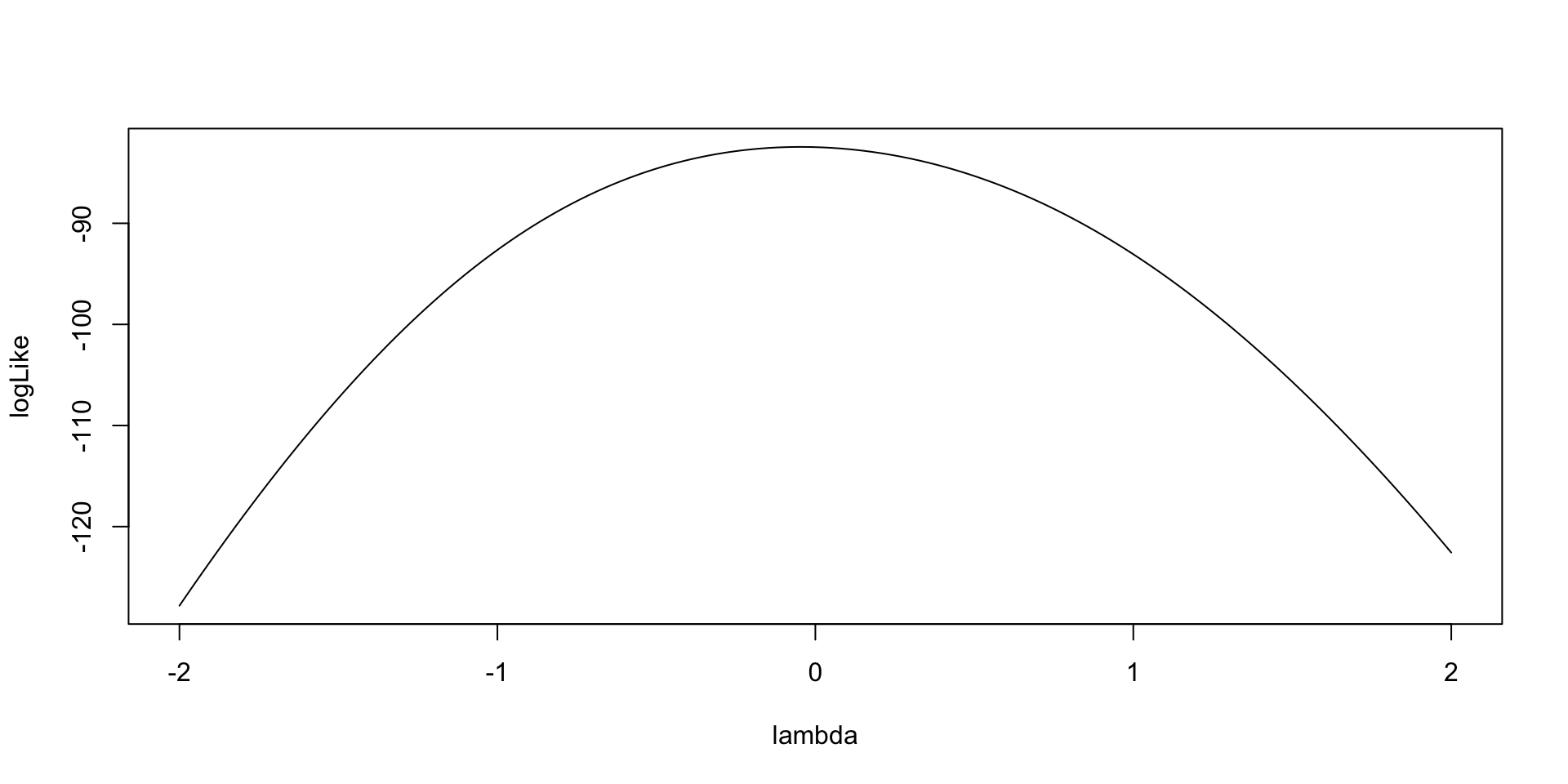
Model (Data) Log Likelihood Functions for \(\theta_p\)

For each person, the same model (data) likelihood function is used

Only now it varies across each item response
Example: Person 1

\[f \left(Y_{1i} \mid \theta_1 \right) = \prod_{i=1}^I \left( \pi_{1i} \right)^{Y_{1i}} \left(1- \pi_{1i} \right)^{1-Y_{1i}}\]

Model (Data) Log Likelihood Functions

As an example for the log-likelihood for \(\theta_2\):

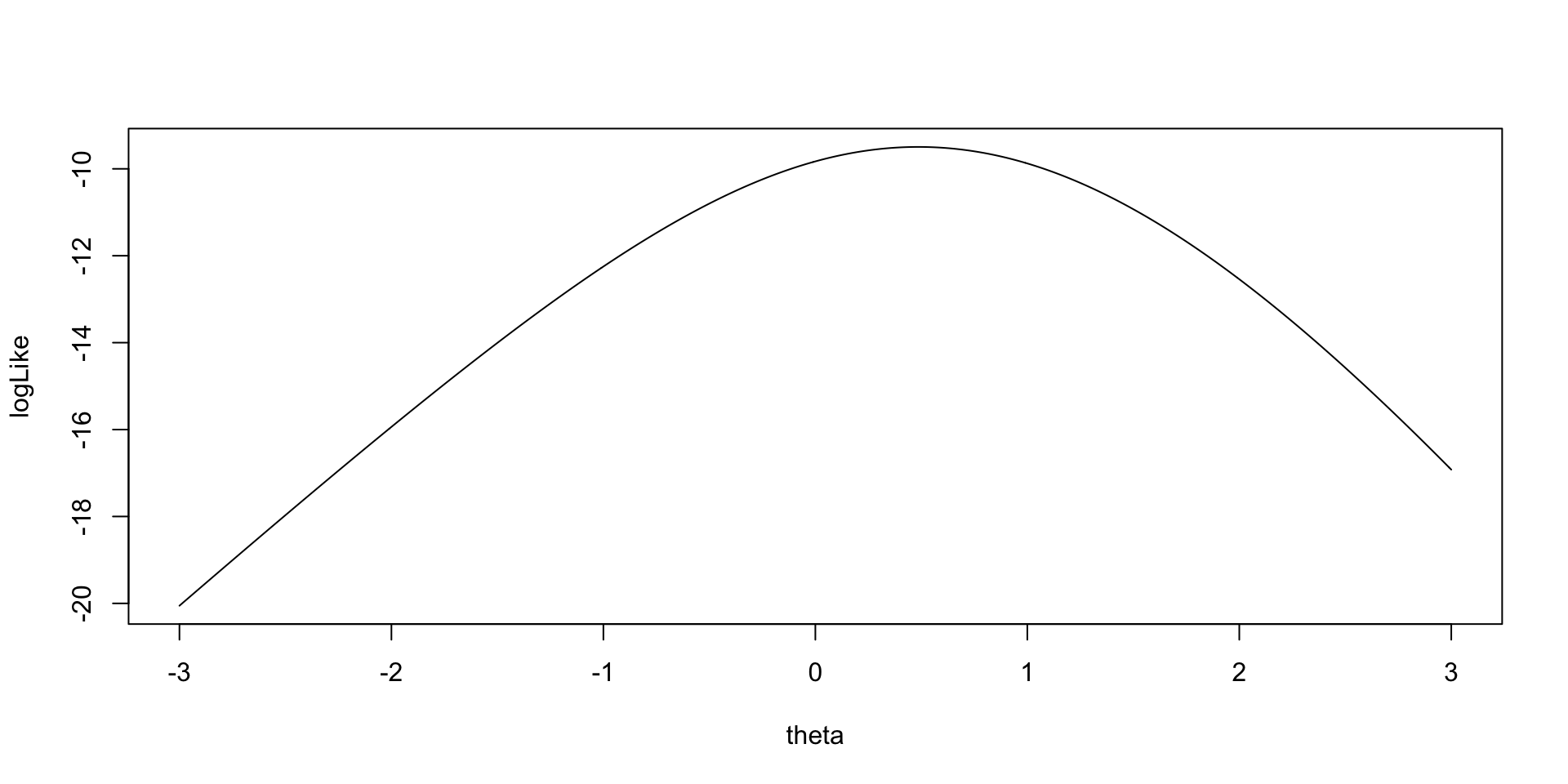
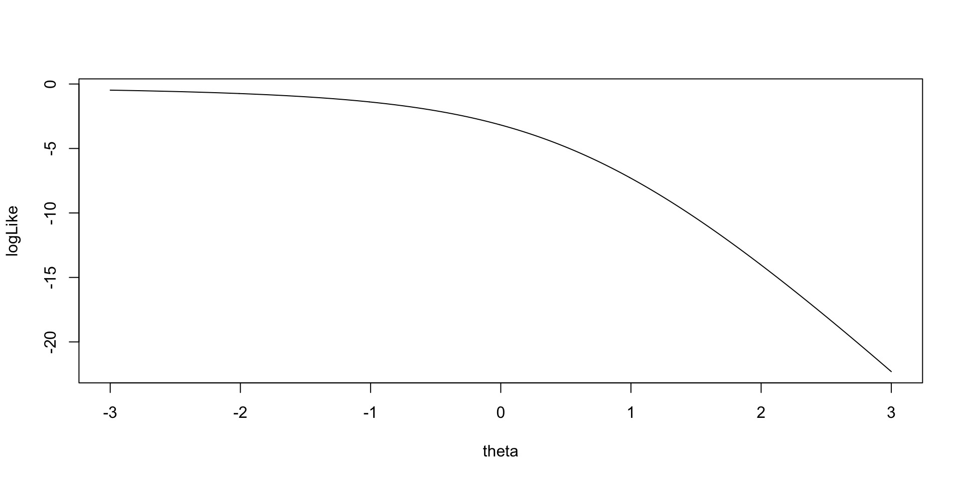
Model (Data) Log Likelihood Functions

As an example for the log-likelihood for \(\theta_1\):

Implementing Bernoulli Outcomes in Stan

Stan’s `model` Block

model {
  
  lambda ~ multi_normal(meanLambda, covLambda); // Prior for item discrimination/factor loadings
  mu ~ multi_normal(meanMu, covMu);             // Prior for item intercepts
  
  theta ~ normal(0, 1);                         // Prior for latent variable (with mean/sd specified)
  
  for (item in 1:nItems){
    Y[item] ~ bernoulli_logit(mu[item] + lambda[item]*theta);
  }
  
}

For logit models without lower/upper asymptote parameters, Stan has a convenient bernoulli_logit() function

Automatically has the link function embedded
The catch: The data have to be defined as an integer

Also, note that there are few differences from the normal outcomes models (CFA)

No \(\psi\) parameters

Stan’s `parameters` Block

parameters {
  vector[nObs] theta;                // the latent variables (one for each person)
  vector[nItems] mu;                 // the item intercepts (one for each item)
  vector[nItems] lambda;             // the factor loadings/item discriminations (one for each item)
}

Only change from normal outcomes (CFA) model:

No \(\psi\) parameters

Stan’s `data {}` Block

data {
  int<lower=0> nObs;                            // number of observations
  int<lower=0> nItems;                          // number of items
  array[nItems, nObs] int<lower=0, upper=1>  Y; // item responses in an array

  vector[nItems] meanMu;             // prior mean vector for intercept parameters
  matrix[nItems, nItems] covMu;      // prior covariance matrix for intercept parameters
  
  vector[nItems] meanLambda;         // prior mean vector for discrimination parameters
  matrix[nItems, nItems] covLambda;  // prior covariance matrix for discrimination parameters
}

One difference from normal outcomes model:

array[nItems, nObs] int<lower=0, upper=1> Y;

Arrays are types of matrices (with more than two dimensions possible)
- Allows for different types of data (here Y are integers)
  - Integer-valued variables needed for bernoulli_logit() function
Arrays are row-major (meaning order of items and persons is switched)
- Can define differently

Change to Data List for Stan Import

The switch of items and observations in the array statement means the data imported have to be transposed:

modelIRT_2PL_SI_data = list(
  nObs = nObs,
  nItems = nItems,
  Y = t(conspiracyItemsDichtomous), 
  meanMu = muMeanVecHP,
  covMu = muCovarianceMatrixHP,
  meanLambda = lambdaMeanVecHP,
  covLambda = lambdaCovarianceMatrixHP
)

Running the Model In Stan

The Stan program takes longer to run than in linear models:

Number of parameters = 197
- 10 observed variables (with two item parameters each: \(\mu_i\) and \(\lambda_i\))
- 177 latent variables (one for each person: 177 parameters)
cmdstanr samples call:

modelIRT_2PL_SI_samples = modelIRT_2PL_SI_stan$sample(
  data = modelIRT_2PL_SI_data,
  seed = 02112022,
  chains = 4,
  parallel_chains = 4,
  iter_warmup = 5000,
  iter_sampling = 5000,
  init = function() list(lambda=rnorm(nItems, mean=5, sd=1))
)

Note: Typically, longer chains are needed for larger models like this
Note: Starting values added (mean of 5 is due to logit function limits)
- Helps keep definition of parameters (stay away from opposite mode)
- Too large of value can lead to NaN values (exceeding numerical precision)

Model Results

Checking convergence with \(\hat{R}\) (PSRF):

[1] 1.002064

Item Parameter Results:

# A tibble: 20 × 10
   variable     mean median     sd    mad     q5    q95  rhat ess_bulk ess_tail
   <chr>       <dbl>  <dbl>  <dbl>  <dbl>  <dbl>  <dbl> <dbl>    <dbl>    <dbl>
 1 mu[1]       -2.47  -2.42  0.464  0.429  -3.32  -1.81  1.00    9127.    8677.
 2 mu[2]       -4.61  -4.44  1.11   1.01   -6.65  -3.12  1.00    8535.    7486.
 3 mu[3]       -4.88  -4.68  1.21   1.07   -7.16  -3.31  1.00    9356.    8119.
 4 mu[4]       -7.05  -6.67  2.19   1.89  -11.1   -4.30  1.00    8270.    7242.
 5 mu[5]      -16.2  -12.3  11.2    6.59  -39.9   -5.94  1.00    4798.    6345.
 6 mu[6]       -6.69  -6.26  2.17   1.77  -10.8   -4.10  1.00    6045.    4830.
 7 mu[7]       -7.21  -6.75  2.33   1.92  -11.6   -4.39  1.00    7341.    6475.
 8 mu[8]      -34.8  -32.2  16.5   16.0   -65.8  -12.8   1.00    9188.   10556.
 9 mu[9]       -7.39  -6.92  2.46   2.01  -11.9   -4.39  1.00    6914.    5954.
10 mu[10]      -5.89  -5.62  1.58   1.42   -8.83  -3.82  1.00    8070.    8124.
11 lambda[1]    1.91   1.86  0.505  0.475   1.18   2.82  1.00    6165.    7147.
12 lambda[2]    3.22   3.08  0.976  0.900   1.90   5.03  1.00    6776.    7092.
13 lambda[3]    2.86   2.71  0.994  0.884   1.54   4.73  1.00    7671.    7519.
14 lambda[4]    4.86   4.57  1.72   1.50    2.68   8.07  1.00    6927.    7033.
15 lambda[5]   13.0    9.87  9.17   5.47    4.60  32.4   1.00    4545.    6646.
16 lambda[6]    4.20   3.88  1.67   1.36    2.17   7.34  1.00    5288.    4401.
17 lambda[7]    4.59   4.28  1.74   1.46    2.43   7.80  1.00    6392.    6464.
18 lambda[8]   21.7   20.0  10.6   10.3     7.55  41.6   1.00    8504.   10234.
19 lambda[9]    5.87   5.50  2.07   1.72    3.33   9.60  1.00    6137.    5651.
20 lambda[10]   3.57   3.38  1.24   1.13    1.93   5.85  1.00    6800.    7093.

Modeling Strategy vs. Didactic Strategy

At this point, one should investigate model fit of the model we just ran

If the model does not fit, then all model parameters could be biased
- Both item parameters and person parameters (\(\theta_p\))
Moreover, the uncertainty accompanying each parameter (the posterior standard deviation) may also be biased
- Especially bad for psychometric models as we quantify reliaiblity with these numbers

But, to teach generalized measurement models, we will first talk about differing models for observed data

Different distributions
Different parameterizations across the different distributions

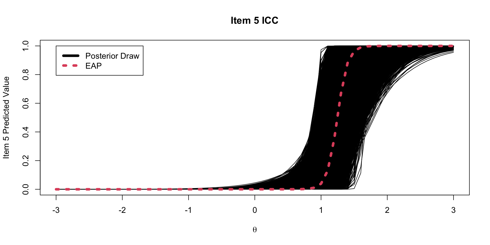
Investigating Item Parameters

One plot that can help provide information about the item parameters is the item characteristic curve (ICC)

The ICC is the plot of the expected value of the response conditional on the value of the latent traits, for a range of latent trait values

\[E \left(Y_{pi} \mid \theta_p \right) = \frac{\exp \left(\mu_{i} +\lambda_{i}\theta_p \right)}{1+\exp \left(\mu_{i} +\lambda_{i}\theta_p \right)} \]

Because we have sampled values for each parameter, we can plot one ICC for each posterior draw

Posterior ICC Plots

Investigating the Item Parameters

Trace plots for \(\mu_i\)

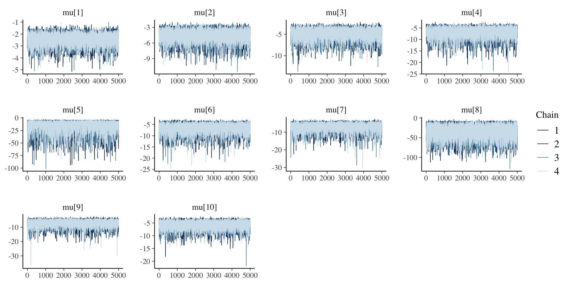
Investigating the Item Parameters

Density plots for \(\mu_i\)

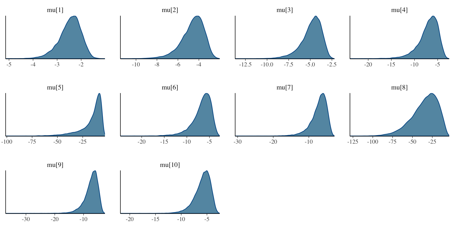
Investigating the Item Parameters

Trace plots for \(\lambda_i\)

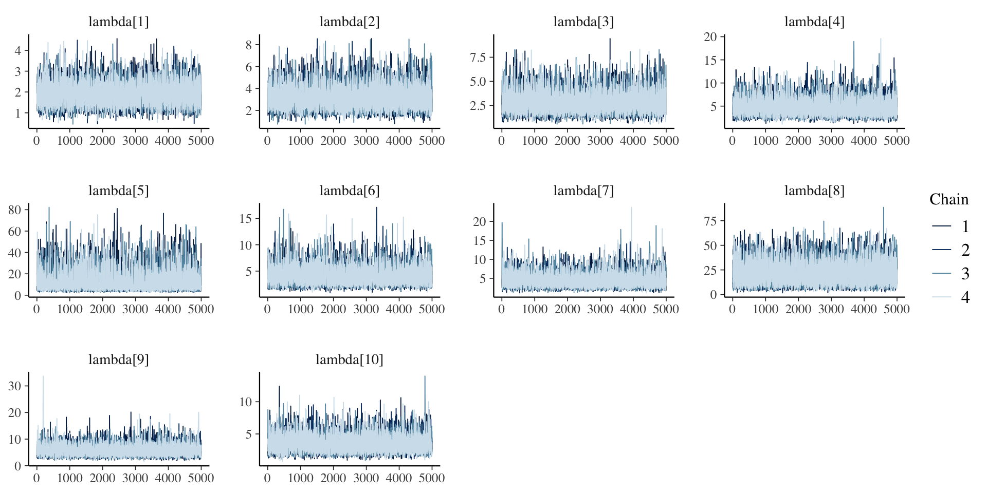
Investigating the Item Parameters

Density plots for \(\lambda_i\)

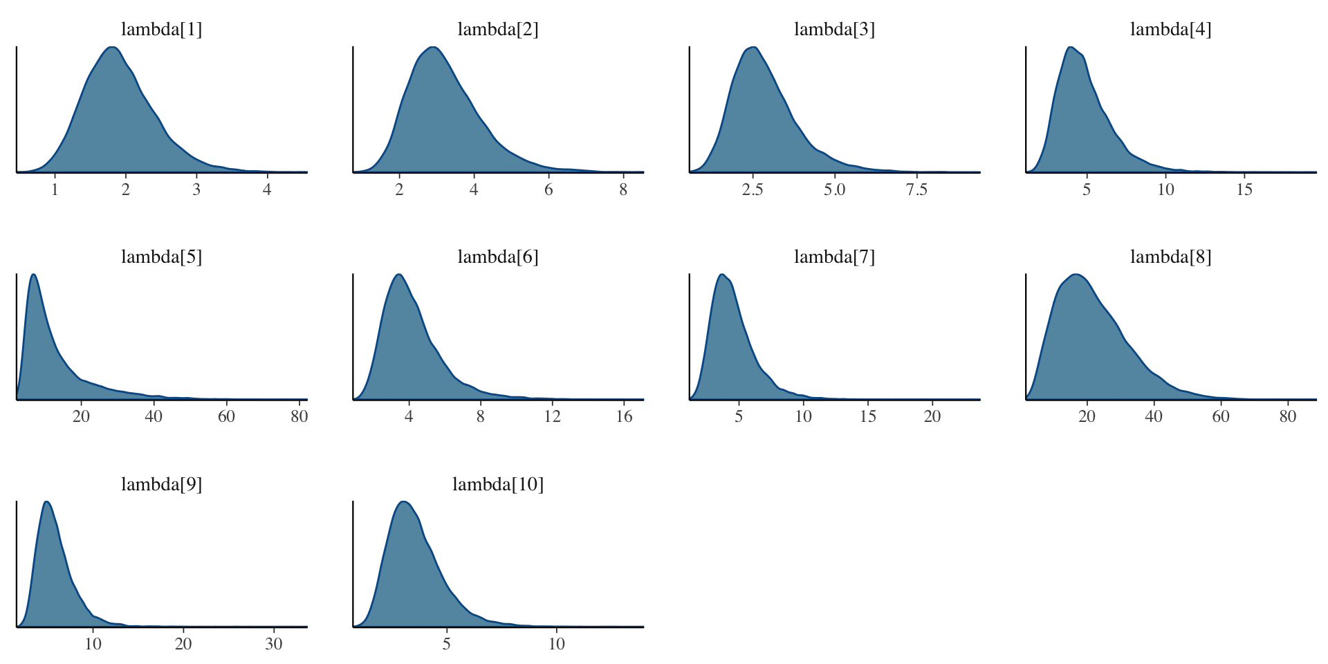
Investigating the Item Parameters

Bivariate plots for \(\mu_i\) and \(\lambda_i\)

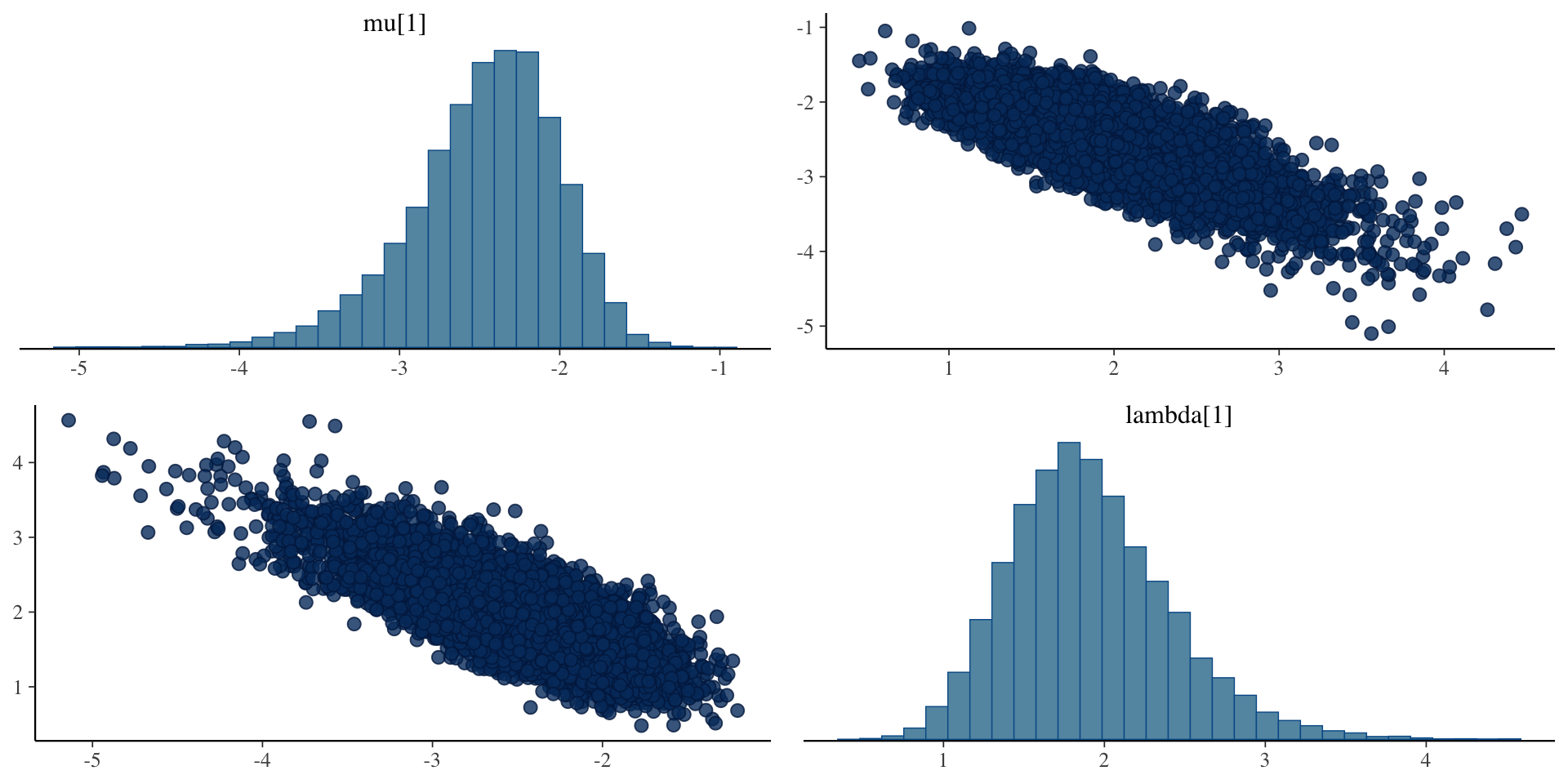
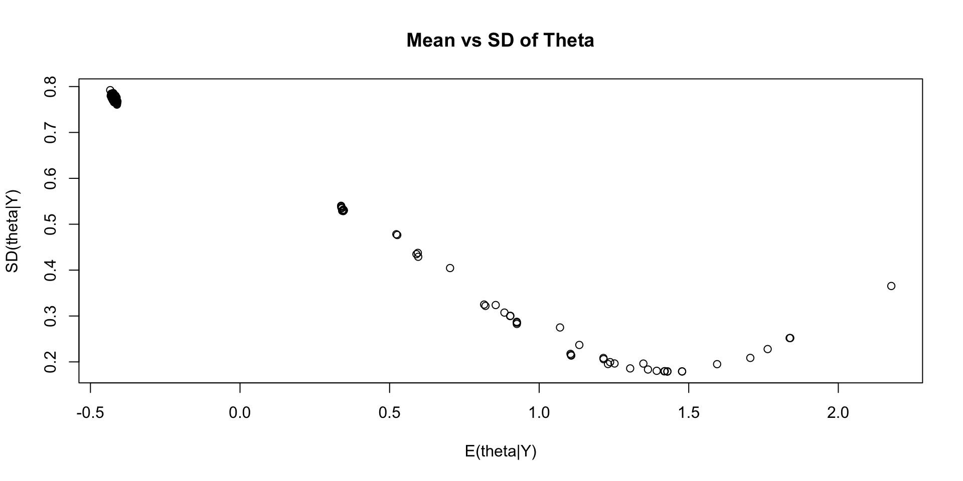
Investigating the Latent Variables

The estimated latent variables are then:

# A tibble: 177 × 10
    variable     mean median    sd   mad      q5   q95  rhat ess_bulk ess_tail
    <chr>       <dbl>  <dbl> <dbl> <dbl>   <dbl> <dbl> <dbl>    <dbl>    <dbl>
  1 theta[1]   -0.419 -0.351 0.771 0.789 -1.79   0.718  1.00   26152.   13351.
  2 theta[2]    1.35   1.34  0.196 0.197  1.03   1.68   1.00    4498.    9571.
  3 theta[3]    1.59   1.59  0.195 0.190  1.28   1.92   1.00    3729.    8562.
  4 theta[4]   -0.419 -0.340 0.773 0.786 -1.81   0.715  1.00   26341.   14493.
  5 theta[5]   -0.418 -0.350 0.768 0.788 -1.79   0.720  1.00   26013.   14259.
  6 theta[6]   -0.418 -0.348 0.774 0.801 -1.80   0.720  1.00   26516.   13446.
  7 theta[7]    0.346  0.430 0.530 0.497 -0.637  1.06   1.00   17933.   11570.
  8 theta[8]    0.594  0.668 0.438 0.391 -0.231  1.16   1.00   13249.   10874.
  9 theta[9]   -0.424 -0.349 0.780 0.802 -1.82   0.721  1.00   29661.   12503.
 10 theta[10]  -0.421 -0.349 0.770 0.788 -1.81   0.713  1.00   27024.   13439.
 11 theta[11]  -0.412 -0.348 0.763 0.785 -1.77   0.720  1.00   25592.   14138.
 12 theta[12]  -0.413 -0.342 0.766 0.770 -1.79   0.709  1.00   24012.   13542.
 13 theta[13]  -0.412 -0.345 0.763 0.774 -1.78   0.715  1.00   28025.   13634.
 14 theta[14]  -0.422 -0.349 0.776 0.797 -1.82   0.723  1.00   26508.   14019.
 15 theta[15]  -0.429 -0.362 0.775 0.797 -1.81   0.706  1.00   27001.   13291.
 16 theta[16]  -0.430 -0.353 0.783 0.793 -1.85   0.714  1.00   25722.   13378.
 17 theta[17]  -0.413 -0.332 0.776 0.787 -1.81   0.720  1.00   26296.   14056.
 18 theta[18]  -0.425 -0.352 0.779 0.789 -1.82   0.726  1.00   27039.   12989.
 19 theta[19]   1.21   1.22  0.209 0.203  0.873  1.55   1.00    5538.    9303.
 20 theta[20]  -0.428 -0.368 0.778 0.801 -1.80   0.730  1.00   25752.   14527.
 21 theta[21]  -0.421 -0.345 0.773 0.787 -1.81   0.716  1.00   26672.   14292.
 22 theta[22]  -0.428 -0.360 0.775 0.789 -1.80   0.724  1.00   24781.   13734.
 23 theta[23]  -0.418 -0.345 0.769 0.791 -1.79   0.721  1.00   27377.   14655.
 24 theta[24]  -0.422 -0.355 0.775 0.800 -1.81   0.708  1.00   27025.   14471.
 25 theta[25]   0.338  0.421 0.540 0.507 -0.664  1.06   1.00   17514.   10223.
 26 theta[26]   1.11   1.12  0.214 0.201  0.746  1.44   1.00    7770.   11481.
 27 theta[27]   0.820  0.865 0.322 0.289  0.225  1.27   1.00   13640.   11242.
 28 theta[28]  -0.412 -0.341 0.770 0.792 -1.78   0.717  1.00   25651.   13909.
 29 theta[29]   0.925  0.958 0.283 0.262  0.413  1.33   1.00   10475.   11618.
 30 theta[30]   1.39   1.39  0.181 0.180  1.10   1.69   1.00    4723.    9137.
 31 theta[31]  -0.420 -0.347 0.778 0.794 -1.81   0.715  1.00   28880.   14632.
 32 theta[32]  -0.416 -0.339 0.777 0.789 -1.82   0.715  1.00   25738.   14394.
 33 theta[33]  -0.417 -0.340 0.777 0.779 -1.81   0.721  1.00   27885.   12687.
 34 theta[34]  -0.415 -0.346 0.767 0.790 -1.78   0.712  1.00   27937.   13696.
 35 theta[35]  -0.429 -0.356 0.777 0.800 -1.82   0.716  1.00   25261.   13641.
 36 theta[36]  -0.420 -0.351 0.769 0.778 -1.79   0.722  1.00   27834.   14394.
 37 theta[37]  -0.423 -0.350 0.783 0.817 -1.81   0.722  1.00   27722.   14583.
 38 theta[38]  -0.422 -0.351 0.778 0.792 -1.83   0.731  1.00   26398.   13262.
 39 theta[39]  -0.426 -0.354 0.785 0.797 -1.83   0.724  1.00   27568.   14170.
 40 theta[40]  -0.420 -0.347 0.782 0.804 -1.82   0.731  1.00   27612.   13180.
 41 theta[41]  -0.422 -0.349 0.770 0.779 -1.80   0.709  1.00   25843.   13866.
 42 theta[42]  -0.424 -0.352 0.785 0.809 -1.83   0.729  1.00   26920.   14393.
 43 theta[43]  -0.426 -0.362 0.784 0.814 -1.83   0.724  1.00   27367.   14238.
 44 theta[44]  -0.411 -0.343 0.765 0.772 -1.78   0.721  1.00   26574.   12757.
 45 theta[45]   1.13   1.16  0.237 0.217  0.713  1.48   1.00    7097.   10907.
 46 theta[46]  -0.421 -0.362 0.766 0.793 -1.79   0.703  1.00   28814.   13644.
 47 theta[47]  -0.428 -0.365 0.778 0.795 -1.81   0.725  1.00   25945.   12836.
 48 theta[48]  -0.424 -0.351 0.782 0.804 -1.82   0.735  1.00   27051.   13772.
 49 theta[49]  -0.431 -0.364 0.780 0.800 -1.82   0.714  1.00   27952.   13794.
 50 theta[50]   0.925  0.959 0.287 0.255  0.411  1.33   1.00   10857.   10658.
 51 theta[51]  -0.428 -0.358 0.784 0.809 -1.83   0.728  1.00   24645.   13000.
 52 theta[52]  -0.412 -0.341 0.768 0.774 -1.80   0.719  1.00   27012.   13655.
 53 theta[53]  -0.424 -0.342 0.777 0.792 -1.82   0.713  1.00   28643.   14009.
 54 theta[54]  -0.414 -0.337 0.772 0.780 -1.79   0.713  1.00   28202.   13873.
 55 theta[55]  -0.416 -0.341 0.780 0.794 -1.82   0.734  1.00   27877.   14147.
 56 theta[56]  -0.421 -0.344 0.779 0.793 -1.82   0.731  1.00   26144.   13752.
 57 theta[57]  -0.415 -0.344 0.772 0.779 -1.81   0.718  1.00   24899.   14011.
 58 theta[58]  -0.423 -0.345 0.775 0.783 -1.82   0.716  1.00   27573.   14458.
 59 theta[59]   0.347  0.427 0.530 0.501 -0.655  1.06   1.00   19314.   12624.
 60 theta[60]  -0.422 -0.351 0.771 0.778 -1.80   0.725  1.00   26424.   12631.
 61 theta[61]   1.25   1.26  0.197 0.188  0.921  1.56   1.00    6249.    9749.
 62 theta[62]  -0.421 -0.357 0.773 0.787 -1.80   0.722  1.00   26427.   13409.
 63 theta[63]  -0.423 -0.353 0.781 0.802 -1.82   0.730  1.00   27558.   12007.
 64 theta[64]   1.10   1.12  0.217 0.204  0.732  1.44   1.00    7983.   11537.
 65 theta[65]  -0.419 -0.343 0.768 0.771 -1.81   0.701  1.00   25226.   13643.
 66 theta[66]  -0.432 -0.360 0.780 0.790 -1.83   0.718  1.00   26087.   14600.
 67 theta[67]  -0.420 -0.345 0.773 0.790 -1.80   0.717  1.00   27069.   13263.
 68 theta[68]  -0.431 -0.350 0.784 0.806 -1.84   0.723  1.00   27200.   15349.
 69 theta[69]  -0.427 -0.363 0.780 0.803 -1.80   0.730  1.00   29034.   14421.
 70 theta[70]  -0.423 -0.356 0.775 0.802 -1.79   0.728  1.00   27479.   13638.
 71 theta[71]  -0.422 -0.344 0.784 0.796 -1.81   0.725  1.00   27794.   14065.
 72 theta[72]   1.30   1.31  0.186 0.181  0.994  1.61   1.00    5829.   10817.
 73 theta[73]  -0.418 -0.360 0.772 0.813 -1.79   0.717  1.00   27530.   14132.
 74 theta[74]  -0.419 -0.342 0.770 0.776 -1.80   0.704  1.00   26746.   13993.
 75 theta[75]  -0.421 -0.351 0.772 0.785 -1.80   0.715  1.00   25773.   14161.
 76 theta[76]   2.18   2.13  0.365 0.350  1.66   2.85   1.00    6634.   11927.
 77 theta[77]  -0.418 -0.347 0.771 0.784 -1.79   0.721  1.00   28920.   13947.
 78 theta[78]   0.816  0.858 0.325 0.295  0.219  1.27   1.00   12856.    9401.
 79 theta[79]   1.22   1.22  0.206 0.201  0.877  1.55   1.00    5478.    9458.
 80 theta[80]  -0.420 -0.360 0.771 0.800 -1.79   0.719  1.00   28275.   14960.
 81 theta[81]  -0.416 -0.344 0.771 0.797 -1.80   0.715  1.00   27267.   13443.
 82 theta[82]  -0.417 -0.349 0.770 0.794 -1.80   0.723  1.00   28376.   13447.
 83 theta[83]  -0.423 -0.355 0.769 0.786 -1.79   0.703  1.00   26611.   14436.
 84 theta[84]   1.48   1.47  0.179 0.178  1.19   1.78   1.00    4294.    8942.
 85 theta[85]   0.590  0.666 0.435 0.389 -0.231  1.16   1.00   13485.   11101.
 86 theta[86]  -0.423 -0.355 0.778 0.805 -1.80   0.725  1.00   27817.   14053.
 87 theta[87]   0.526  0.611 0.476 0.435 -0.368  1.15   1.00   13565.   11342.
 88 theta[88]  -0.415 -0.346 0.767 0.775 -1.78   0.718  1.00   28371.   13831.
 89 theta[89]  -0.423 -0.350 0.778 0.795 -1.80   0.720  1.00   27809.   14209.
 90 theta[90]   0.345  0.432 0.532 0.494 -0.662  1.06   1.00   18369.   12549.
 91 theta[91]  -0.426 -0.363 0.770 0.800 -1.79   0.714  1.00   27819.   14382.
 92 theta[92]   1.24   1.24  0.199 0.189  0.903  1.55   1.00    6266.   10135.
 93 theta[93]  -0.425 -0.348 0.782 0.792 -1.81   0.720  1.00   24971.   13234.
 94 theta[94]   1.84   1.81  0.252 0.238  1.47   2.29   1.00    4280.    8553.
 95 theta[95]   1.42   1.42  0.179 0.178  1.13   1.72   1.00    4190.    9508.
 96 theta[96]  -0.418 -0.345 0.777 0.800 -1.80   0.733  1.00   26791.   13729.
 97 theta[97]  -0.416 -0.344 0.780 0.794 -1.81   0.731  1.00   26977.   13640.
 98 theta[98]  -0.427 -0.361 0.779 0.793 -1.82   0.717  1.00   25786.   13457.
 99 theta[99]  -0.423 -0.348 0.779 0.790 -1.82   0.718  1.00   28603.   13849.
100 theta[100] -0.423 -0.351 0.778 0.800 -1.80   0.719  1.00   28349.   14408.
101 theta[101] -0.424 -0.346 0.782 0.794 -1.83   0.721  1.00   26289.   13158.
102 theta[102]  1.76   1.75  0.228 0.217  1.42   2.17   1.00    4056.    8813.
103 theta[103] -0.420 -0.358 0.774 0.784 -1.81   0.721  1.00   25295.   13046.
104 theta[104]  1.43   1.42  0.180 0.177  1.14   1.73   1.00    4359.    8532.
105 theta[105] -0.416 -0.347 0.771 0.787 -1.80   0.707  1.00   26705.   13928.
106 theta[106]  0.904  0.945 0.300 0.269  0.353  1.32   1.00    9497.    9933.
107 theta[107]  1.48   1.47  0.179 0.178  1.19   1.78   1.00    4382.    8967.
108 theta[108]  0.339  0.426 0.536 0.498 -0.678  1.05   1.00   17189.   11203.
109 theta[109] -0.428 -0.362 0.777 0.792 -1.82   0.720  1.00   25012.   12911.
110 theta[110] -0.422 -0.349 0.776 0.805 -1.82   0.712  1.00   28059.   14145.
111 theta[111] -0.422 -0.355 0.771 0.795 -1.79   0.718  1.00   25719.   13244.
112 theta[112]  0.338  0.417 0.539 0.503 -0.684  1.06   1.00   18740.   11555.
113 theta[113] -0.422 -0.357 0.776 0.799 -1.80   0.735  1.00   27301.   13201.
114 theta[114] -0.422 -0.350 0.770 0.785 -1.80   0.714  1.00   24473.   14262.
115 theta[115]  1.43   1.43  0.179 0.176  1.14   1.72   1.00    4575.    8921.
116 theta[116] -0.419 -0.349 0.776 0.796 -1.82   0.717  1.00   25987.   14703.
117 theta[117] -0.417 -0.351 0.766 0.780 -1.80   0.715  1.00   26309.   15028.
118 theta[118] -0.418 -0.342 0.779 0.796 -1.83   0.727  1.00   29358.   14514.
119 theta[119] -0.416 -0.344 0.772 0.790 -1.81   0.714  1.00   27990.   14315.
120 theta[120] -0.410 -0.337 0.768 0.781 -1.79   0.710  1.00   27590.   14513.
121 theta[121]  0.702  0.770 0.404 0.360 -0.0640 1.23   1.00   10168.   11382.
122 theta[122]  0.341  0.421 0.529 0.499 -0.653  1.05   1.00   19173.   11741.
123 theta[123] -0.419 -0.348 0.771 0.787 -1.79   0.728  1.00   27405.   14062.
124 theta[124] -0.425 -0.356 0.775 0.796 -1.81   0.726  1.00   26746.   13820.
125 theta[125] -0.415 -0.349 0.765 0.786 -1.78   0.712  1.00   25415.   13794.
126 theta[126]  0.341  0.427 0.535 0.505 -0.664  1.05   1.00   18718.   11305.
127 theta[127]  0.903  0.939 0.300 0.269  0.360  1.32   1.00   10506.   10082.
128 theta[128] -0.428 -0.355 0.784 0.794 -1.84   0.720  1.00   25555.   14072.
129 theta[129] -0.420 -0.349 0.778 0.792 -1.81   0.728  1.00   27309.   13622.
130 theta[130]  1.71   1.69  0.209 0.202  1.39   2.07   1.00    3778.    8275.
131 theta[131]  0.345  0.433 0.530 0.490 -0.660  1.05   1.00   18408.   12102.
132 theta[132]  1.42   1.42  0.180 0.178  1.13   1.72   1.00    4599.    8064.
133 theta[133] -0.417 -0.349 0.769 0.789 -1.79   0.718  1.00   26912.   14602.
134 theta[134]  1.84   1.81  0.252 0.237  1.47   2.29   1.00    4435.    8055.
135 theta[135] -0.411 -0.342 0.761 0.782 -1.77   0.711  1.00   26172.   13873.
136 theta[136] -0.415 -0.344 0.770 0.790 -1.79   0.721  1.00   26516.   13876.
137 theta[137] -0.418 -0.350 0.771 0.794 -1.78   0.719  1.00   28030.   14685.
138 theta[138] -0.424 -0.348 0.786 0.805 -1.83   0.735  1.00   26584.   13290.
139 theta[139] -0.423 -0.352 0.769 0.788 -1.81   0.716  1.00   28754.   13883.
140 theta[140]  0.596  0.668 0.429 0.390 -0.219  1.17   1.00   13672.   11664.
141 theta[141] -0.427 -0.356 0.783 0.794 -1.82   0.721  1.00   26164.   12134.
142 theta[142] -0.420 -0.348 0.782 0.795 -1.82   0.735  1.00   27725.   13527.
143 theta[143] -0.417 -0.344 0.775 0.786 -1.81   0.713  1.00   26121.   14073.
144 theta[144] -0.424 -0.353 0.779 0.789 -1.83   0.725  1.00   26597.   13181.
145 theta[145] -0.424 -0.352 0.779 0.797 -1.81   0.723  1.00   25228.   13780.
146 theta[146] -0.421 -0.351 0.771 0.794 -1.80   0.722  1.00   26727.   14300.
147 theta[147] -0.416 -0.348 0.770 0.789 -1.79   0.712  1.00   28198.   13408.
148 theta[148]  1.23   1.23  0.195 0.189  0.910  1.55   1.00    5606.   10815.
149 theta[149] -0.428 -0.358 0.775 0.788 -1.82   0.720  1.00   25374.   13597.
150 theta[150] -0.423 -0.348 0.772 0.789 -1.81   0.710  1.00   26342.   13888.
151 theta[151]  0.345  0.428 0.529 0.497 -0.649  1.05   1.00   17907.   11271.
152 theta[152] -0.424 -0.354 0.778 0.804 -1.80   0.727  1.00   28455.   13417.
153 theta[153]  1.36   1.36  0.183 0.180  1.06   1.67   1.00    4914.   10037.
154 theta[154] -0.416 -0.344 0.777 0.796 -1.79   0.722  1.00   25826.   12953.
155 theta[155] -0.419 -0.351 0.770 0.789 -1.79   0.721  1.00   26638.   14070.
156 theta[156] -0.422 -0.357 0.769 0.790 -1.79   0.720  1.00   27698.   13760.
157 theta[157] -0.419 -0.353 0.774 0.790 -1.80   0.726  1.00   26001.   13076.
158 theta[158] -0.426 -0.345 0.784 0.798 -1.85   0.712  1.00   27149.   14062.
159 theta[159]  1.07   1.11  0.275 0.241  0.569  1.45   1.00    7353.    9955.
160 theta[160] -0.416 -0.346 0.774 0.795 -1.79   0.722  1.00   27394.   14460.
161 theta[161]  0.884  0.924 0.307 0.276  0.317  1.31   1.00    9998.   10489.
162 theta[162]  0.523  0.606 0.478 0.428 -0.385  1.14   1.00   14350.   11197.
163 theta[163] -0.425 -0.357 0.772 0.789 -1.78   0.714  1.00   25663.   13413.
164 theta[164] -0.416 -0.344 0.772 0.787 -1.81   0.714  1.00   25919.   13289.
165 theta[165]  0.926  0.960 0.286 0.260  0.413  1.33   1.00   10494.    9885.
166 theta[166] -0.429 -0.354 0.784 0.799 -1.84   0.725  1.00   28883.   13803.
167 theta[167] -0.426 -0.354 0.781 0.801 -1.81   0.728  1.00   27570.   13493.
168 theta[168]  1.11   1.12  0.215 0.201  0.742  1.44   1.00    7696.   11171.
169 theta[169] -0.425 -0.351 0.776 0.788 -1.82   0.710  1.00   26964.   14428.
170 theta[170] -0.421 -0.346 0.774 0.787 -1.81   0.708  1.00   28620.   15397.
171 theta[171]  0.855  0.900 0.324 0.291  0.256  1.29   1.00   10595.   10843.
172 theta[172] -0.434 -0.361 0.792 0.805 -1.87   0.728  1.00   25038.   13132.
173 theta[173] -0.420 -0.345 0.781 0.804 -1.81   0.729  1.00   26334.   14305.
174 theta[174] -0.423 -0.352 0.778 0.788 -1.82   0.725  1.00   25626.   14439.
175 theta[175] -0.420 -0.345 0.767 0.778 -1.79   0.710  1.00   25726.   13002.
176 theta[176] -0.420 -0.356 0.769 0.783 -1.78   0.720  1.00   26782.   14100.
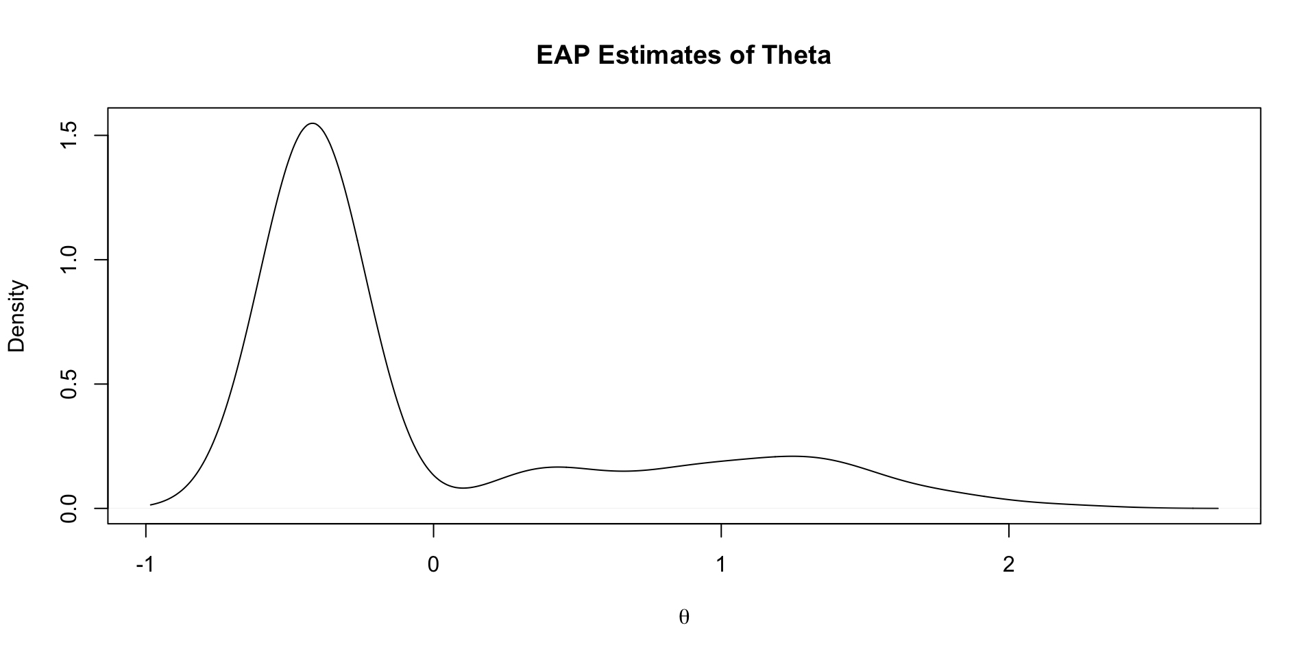
177 theta[177] -0.416 -0.347 0.771 0.793 -1.81   0.723  1.00   25489.   13747.

EAP Estimates of Latent Variables

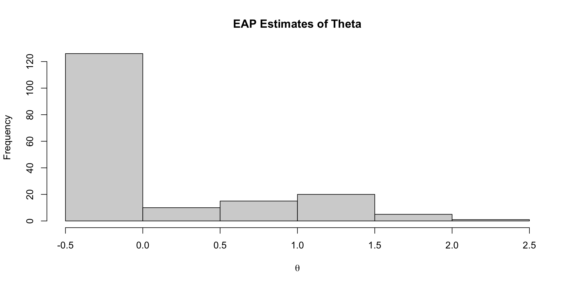
Density of EAP Estimates

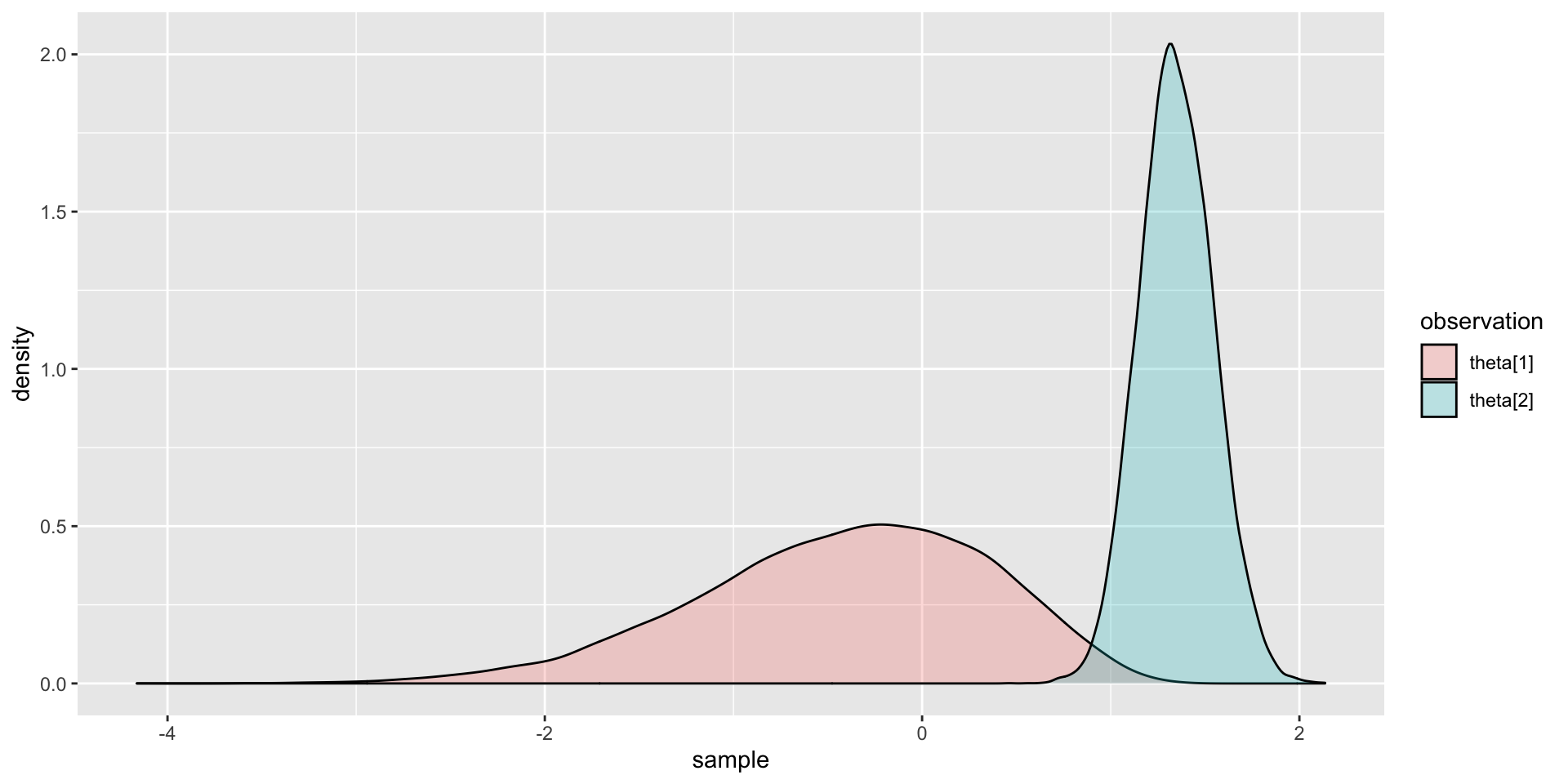
Comparing Two Posterior Distributions

Comparing EAP Estimates with Posterior SDs

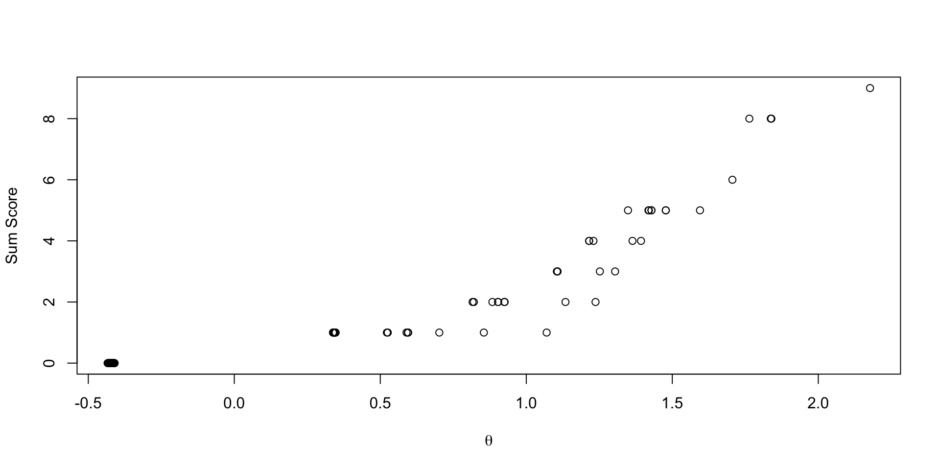
Comparing EAP Estimates with Sum Score

Discrimination/Difficulty Parameterization

The slope/intercept form is used in many model families:

Confirmatory factor analysis
Item factor analysis
Multidimensional item response theory

In educational measurement, a more common form of the model is discrimination/difficulty:

\[logit \left( P\left( Y_{pi}=1 \mid \theta_p \right) \right) = a_i\left(\theta_p - b_i\right)\]

More commonly, this is expressed on the data scale:

\[P\left( Y_{pi}=1 \mid \theta_p \right) = \frac{\exp \left( a_i\left(\theta_p - b_i\right) \right)}{1+\exp \left(a_i\left(\theta_p - b_i\right) \right)} \]

Comparisons of Parameterizations

We’ve mentioned before there is a one-one relationship between the models:

\[a_i\left(\theta_p - b_i\right) = -a_i b_i + a_i\theta_p = \mu_i + \lambda_i\theta_p\]

Where:

\(\mu_i = -a_ib_i\)
\(\lambda_i = a_i\)

Alternatively:

\(b_i = -\frac{\mu_i}{a_i}\)
\(a_i = \lambda_i\)

Calculating Discrimination/Difficulty Parameters in Generated Quantities

We can calculate one parameterization from the other using Stan’s generated quantities:

generated quantities{
  vector[nItems] a;
  vector[nItems] b;
  
  for (item in 1:nItems){
    a[item] = lambda[item];
    b[item] = -1*mu[item]/lambda[item];
  }
  
}

Discrimination/Difficulty Parameter Estimates

# A tibble: 20 × 10
   variable  mean median     sd    mad    q5   q95  rhat ess_bulk ess_tail
   <chr>    <dbl>  <dbl>  <dbl>  <dbl> <dbl> <dbl> <dbl>    <dbl>    <dbl>
 1 a[1]      1.90   1.85  0.508  0.483  1.16  2.80  1.00    5416.    7254.
 2 a[2]      3.22   3.08  0.993  0.891  1.87  5.03  1.00    6021.    6110.
 3 a[3]      2.86   2.72  0.988  0.893  1.52  4.70  1.00    5245.    5770.
 4 a[4]      4.84   4.52  1.77   1.51   2.63  8.17  1.00    5104.    4819.
 5 a[5]     13.2    9.89  9.58   5.55   4.51 33.3   1.00    3475.    4184.
 6 a[6]      4.17   3.85  1.69   1.36   2.17  7.22  1.00    4633.    4016.
 7 a[7]      4.58   4.24  1.76   1.45   2.43  7.81  1.00    5174.    4715.
 8 a[8]     21.9   20.4  10.5   10.4    7.63 41.5   1.00    7152.    8512.
 9 a[9]      5.82   5.44  2.09   1.71   3.29  9.57  1.00    5607.    5254.
10 a[10]     3.60   3.38  1.29   1.11   1.95  5.97  1.00    4870.    5218.
11 b[1]      1.34   1.31  0.252  0.222  1.00  1.80  1.00    4751.    8560.
12 b[2]      1.47   1.45  0.206  0.188  1.18  1.84  1.00    3600.    6074.
13 b[3]      1.79   1.73  0.326  0.266  1.38  2.36  1.00    4206.    6396.
14 b[4]      1.49   1.48  0.178  0.165  1.22  1.80  1.00    2758.    5396.
15 b[5]      1.27   1.26  0.128  0.127  1.06  1.49  1.00    2355.    4835.
16 b[6]      1.65   1.63  0.230  0.209  1.34  2.06  1.00    3082.    5070.
17 b[7]      1.62   1.60  0.207  0.191  1.32  1.99  1.00    3233.    5991.
18 b[8]      1.63   1.62  0.161  0.159  1.37  1.89  1.00    2096.    4027.
19 b[9]      1.28   1.27  0.138  0.135  1.06  1.51  1.00    2627.    5608.
20 b[10]     1.71   1.67  0.254  0.224  1.36  2.15  1.00    3488.    5181.

Estimating the Discrimination/Difficulty Model

A change is needed to Stan’s model statement to directly estimate the discrimination/difficulty model:

model {
  
  a ~ multi_normal(meanA, covA); // Prior for item discrimination/factor loadings
  b ~ multi_normal(meanB, covB);             // Prior for item intercepts
  
  theta ~ normal(0, 1);                         // Prior for latent variable (with mean/sd specified)
  
  for (item in 1:nItems){
    Y[item] ~ bernoulli_logit(a[item]*(theta - b[item]));
  }
  
}

We can also estimate the slope/intercept parameters from the discrimination/difficulty parameters:

generated quantities{
  vector[nItems] lambda;
  vector[nItems] mu;
  
  lambda = a;
  for (item in 1:nItems){
    mu[item] = -1*a[item]*b[item];
  }
}

Model Results

Checking convergence:

[1] 1.002703

Checking parameter estimates:

# A tibble: 20 × 10
   variable  mean median     sd    mad    q5   q95  rhat ess_bulk ess_tail
   <chr>    <dbl>  <dbl>  <dbl>  <dbl> <dbl> <dbl> <dbl>    <dbl>    <dbl>
 1 a[1]      1.63   1.60  0.443  0.424 0.984  2.42  1.00    4257.    6633.
 2 a[2]      2.72   2.60  0.822  0.734 1.61   4.19  1.00    4810.    7125.
 3 a[3]      2.30   2.19  0.769  0.707 1.25   3.69  1.00    6232.    8591.
 4 a[4]      3.92   3.69  1.35   1.18  2.18   6.41  1.00    4815.    6879.
 5 a[5]     11.6    7.52 11.4    4.05  3.62  36.2   1.00    2113.    1388.
 6 a[6]      3.26   3.07  1.19   1.04  1.70   5.41  1.00    3763.    5474.
 7 a[7]      3.56   3.35  1.28   1.11  1.92   5.90  1.00    4833.    5485.
 8 a[8]     27.8   23.8  17.8   16.9   6.39  61.8   1.00    5003.    3860.
 9 a[9]      4.68   4.43  1.48   1.31  2.76   7.45  1.00    4695.    5613.
10 a[10]     2.83   2.69  0.972  0.875 1.55   4.57  1.00    5581.    7733.
11 b[1]      1.48   1.44  0.313  0.261 1.08   2.02  1.00    3615.    5512.
12 b[2]      1.60   1.57  0.238  0.214 1.26   2.03  1.00    3158.    6129.
13 b[3]      2.01   1.94  0.392  0.318 1.52   2.71  1.00    4417.    7589.
14 b[4]      1.61   1.60  0.201  0.186 1.32   1.98  1.00    2857.    5543.
15 b[5]      1.34   1.34  0.141  0.137 1.13   1.58  1.00    1782.    1076.
16 b[6]      1.84   1.79  0.307  0.251 1.45   2.36  1.00    2958.    4921.
17 b[7]      1.79   1.76  0.252  0.228 1.44   2.25  1.00    2924.    5063.
18 b[8]      1.76   1.76  0.168  0.167 1.50   2.05  1.00    1884.    3290.
19 b[9]      1.36   1.36  0.154  0.151 1.12   1.62  1.00    2460.    5657.
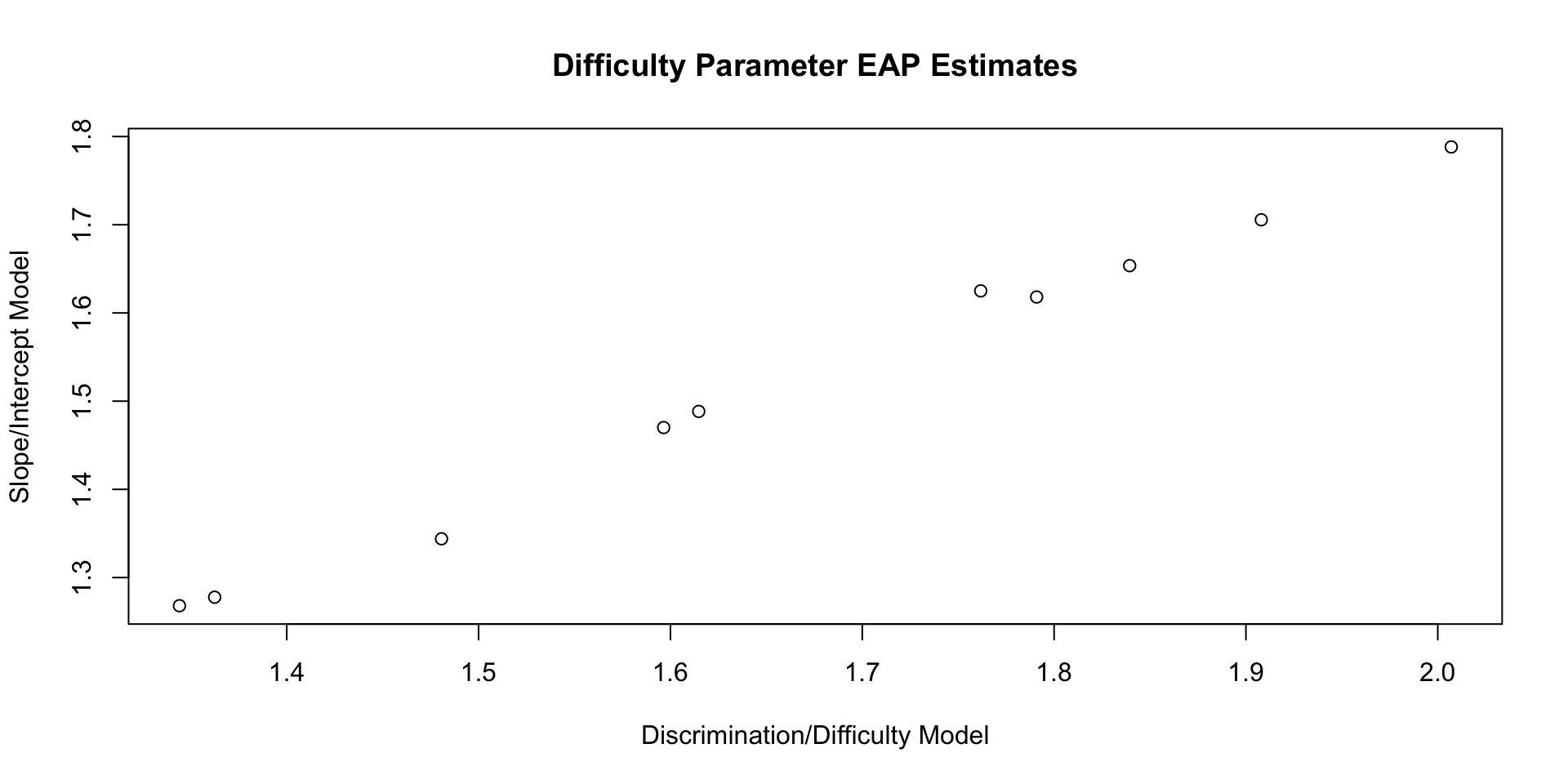
20 b[10]     1.91   1.86  0.323  0.269 1.49   2.46  1.00    3324.    6455.

Comparing Difficulty Parameters

Difficulty parameters from discrimination/difficulty model:

# A tibble: 10 × 10
   variable  mean median    sd   mad    q5   q95  rhat ess_bulk ess_tail
   <chr>    <dbl>  <dbl> <dbl> <dbl> <dbl> <dbl> <dbl>    <dbl>    <dbl>
 1 b[1]      1.48   1.44 0.313 0.261  1.08  2.02  1.00    3615.    5512.
 2 b[2]      1.60   1.57 0.238 0.214  1.26  2.03  1.00    3158.    6129.
 3 b[3]      2.01   1.94 0.392 0.318  1.52  2.71  1.00    4417.    7589.
 4 b[4]      1.61   1.60 0.201 0.186  1.32  1.98  1.00    2857.    5543.
 5 b[5]      1.34   1.34 0.141 0.137  1.13  1.58  1.00    1782.    1076.
 6 b[6]      1.84   1.79 0.307 0.251  1.45  2.36  1.00    2958.    4921.
 7 b[7]      1.79   1.76 0.252 0.228  1.44  2.25  1.00    2924.    5063.
 8 b[8]      1.76   1.76 0.168 0.167  1.50  2.05  1.00    1884.    3290.
 9 b[9]      1.36   1.36 0.154 0.151  1.12  1.62  1.00    2460.    5657.
10 b[10]     1.91   1.86 0.323 0.269  1.49  2.46  1.00    3324.    6455.

Difficulty parameters from slope/intercept model:

# A tibble: 10 × 10
   variable  mean median    sd   mad    q5   q95  rhat ess_bulk ess_tail
   <chr>    <dbl>  <dbl> <dbl> <dbl> <dbl> <dbl> <dbl>    <dbl>    <dbl>
 1 b[1]      1.34   1.31 0.252 0.222  1.00  1.80  1.00    4751.    8560.
 2 b[2]      1.47   1.45 0.206 0.188  1.18  1.84  1.00    3600.    6074.
 3 b[3]      1.79   1.73 0.326 0.266  1.38  2.36  1.00    4206.    6396.
 4 b[4]      1.49   1.48 0.178 0.165  1.22  1.80  1.00    2758.    5396.
 5 b[5]      1.27   1.26 0.128 0.127  1.06  1.49  1.00    2355.    4835.
 6 b[6]      1.65   1.63 0.230 0.209  1.34  2.06  1.00    3082.    5070.
 7 b[7]      1.62   1.60 0.207 0.191  1.32  1.99  1.00    3233.    5991.
 8 b[8]      1.63   1.62 0.161 0.159  1.37  1.89  1.00    2096.    4027.
 9 b[9]      1.28   1.27 0.138 0.135  1.06  1.51  1.00    2627.    5608.
10 b[10]     1.71   1.67 0.254 0.224  1.36  2.15  1.00    3488.    5181.

Comparing Difficulty Parameters: Plot

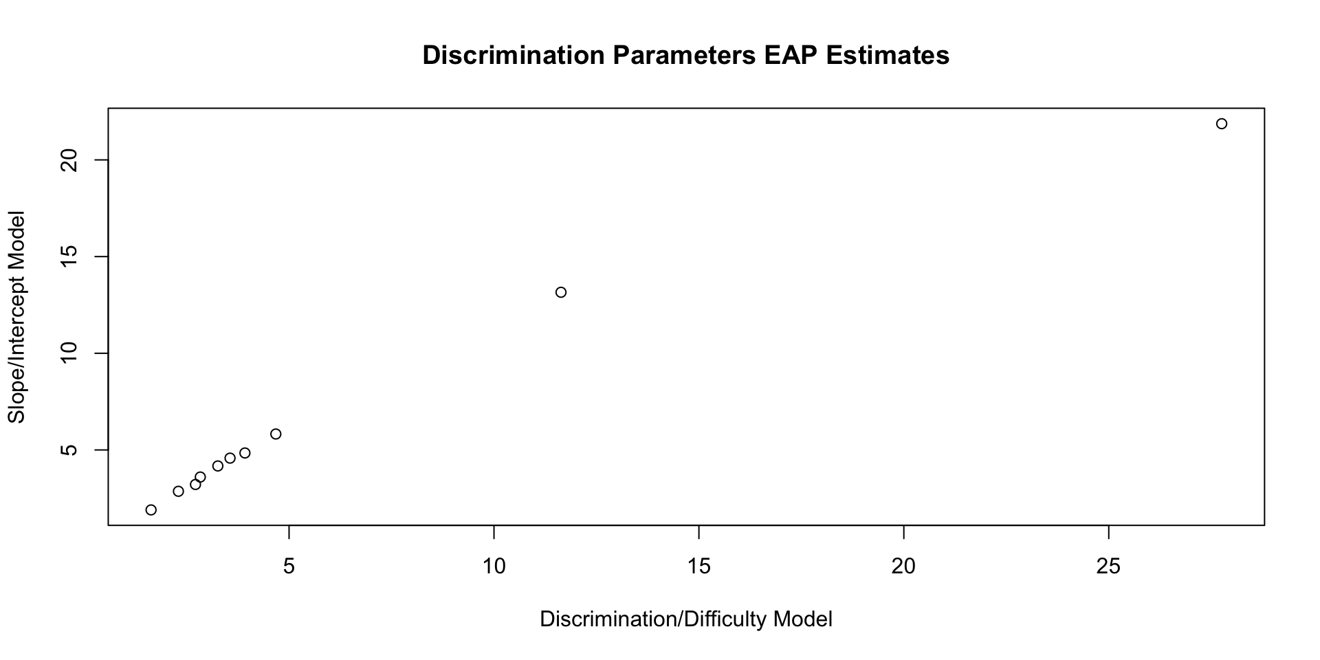
Comparing Discrimination Parameters

Discrimination parameters from discrimination/difficulty model:

# A tibble: 10 × 10
   variable  mean median     sd    mad    q5   q95  rhat ess_bulk ess_tail
   <chr>    <dbl>  <dbl>  <dbl>  <dbl> <dbl> <dbl> <dbl>    <dbl>    <dbl>
 1 a[1]      1.63   1.60  0.443  0.424 0.984  2.42  1.00    4257.    6633.
 2 a[2]      2.72   2.60  0.822  0.734 1.61   4.19  1.00    4810.    7125.
 3 a[3]      2.30   2.19  0.769  0.707 1.25   3.69  1.00    6232.    8591.
 4 a[4]      3.92   3.69  1.35   1.18  2.18   6.41  1.00    4815.    6879.
 5 a[5]     11.6    7.52 11.4    4.05  3.62  36.2   1.00    2113.    1388.
 6 a[6]      3.26   3.07  1.19   1.04  1.70   5.41  1.00    3763.    5474.
 7 a[7]      3.56   3.35  1.28   1.11  1.92   5.90  1.00    4833.    5485.
 8 a[8]     27.8   23.8  17.8   16.9   6.39  61.8   1.00    5003.    3860.
 9 a[9]      4.68   4.43  1.48   1.31  2.76   7.45  1.00    4695.    5613.
10 a[10]     2.83   2.69  0.972  0.875 1.55   4.57  1.00    5581.    7733.

Discrimination parameters from slope/intercept model:

# A tibble: 10 × 10
   variable  mean median     sd    mad    q5   q95  rhat ess_bulk ess_tail
   <chr>    <dbl>  <dbl>  <dbl>  <dbl> <dbl> <dbl> <dbl>    <dbl>    <dbl>
 1 a[1]      1.90   1.85  0.508  0.483  1.16  2.80  1.00    5416.    7254.
 2 a[2]      3.22   3.08  0.993  0.891  1.87  5.03  1.00    6021.    6110.
 3 a[3]      2.86   2.72  0.988  0.893  1.52  4.70  1.00    5245.    5770.
 4 a[4]      4.84   4.52  1.77   1.51   2.63  8.17  1.00    5104.    4819.
 5 a[5]     13.2    9.89  9.58   5.55   4.51 33.3   1.00    3475.    4184.
 6 a[6]      4.17   3.85  1.69   1.36   2.17  7.22  1.00    4633.    4016.
 7 a[7]      4.58   4.24  1.76   1.45   2.43  7.81  1.00    5174.    4715.
 8 a[8]     21.9   20.4  10.5   10.4    7.63 41.5   1.00    7152.    8512.
 9 a[9]      5.82   5.44  2.09   1.71   3.29  9.57  1.00    5607.    5254.
10 a[10]     3.60   3.38  1.29   1.11   1.95  5.97  1.00    4870.    5218.

Comparing Discrimination Parameters: Plot

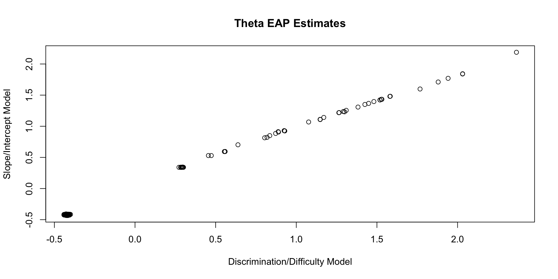
Comparing Theta EAP Estimates

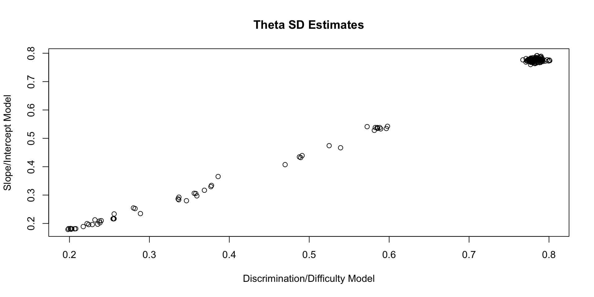
Comparing Theta SD Estimates

Posterior Distributions Are Different

Although the parameters of each type of model can be found from the others, the posterior distributions are not the same

Prior distributions are defined on the coded model parameters
Posterior distributions are not necessarily the same
- But are linearly related (in this case)
More extreme choices of priors would lead to more extreme differences

Estimating IRT Model Auxiliary Statistics

We can also use the generated quantities block to estimate some important auxiliary statitics from IRT models

Test characteristic curve estimates (with posterior standard deviations); TCC
Item information functions (with posterior standard deviations); IIF
Test information functions (with posterior standard deviations); TIF

Shown for the discrimination/difficulty parameterization (but applies to slope/intercept, too)

The key:

Define a set of \(\theta\) values and import them into Stan
Then calculate each statistic using (conditional on) each value of \(\theta\) imported

Range of \(\theta\)

To begin, define a range of \(\theta\) over which you wish to calculate these statistics

As we’ve used a standardized \(\theta\), we can define that range being from \(\[-3, 3\]\)
- Covers about 99% of the distribution of \(\theta\)
Here, I am creating a sequence that adds .01 to each successive values (only first 10 shown)
- Makes for better plots
- More values (smaller interval) slows the estimation process down
- More values also takes more memory to store chains

thetaVals = seq(-3,3,.01)
thetaVals[1:10]

 [1] -3.00 -2.99 -2.98 -2.97 -2.96 -2.95 -2.94 -2.93 -2.92 -2.91

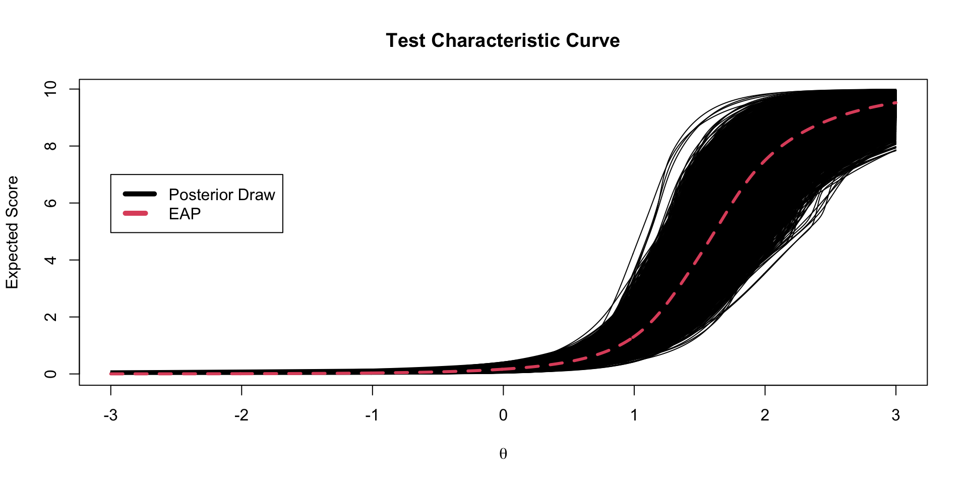
Test Characteristic Curves

The test characteristic curve is formed by taking the sum of the expected value for each item, conditional on a value of \(\theta\)

\[TCC(\theta) = \sum_{i=1}^I \frac{\exp \left(a_i \left(\theta -b_i \right) \right)}{1+ \exp \left(a_i \left(\theta-b_i \right) \right)}\]

We must compute this for each imported value of \(\theta\) across all iterations of the Markov Chain

TCC Plots

Each TCC theta-to-raw score conversion has its own posterior standard error

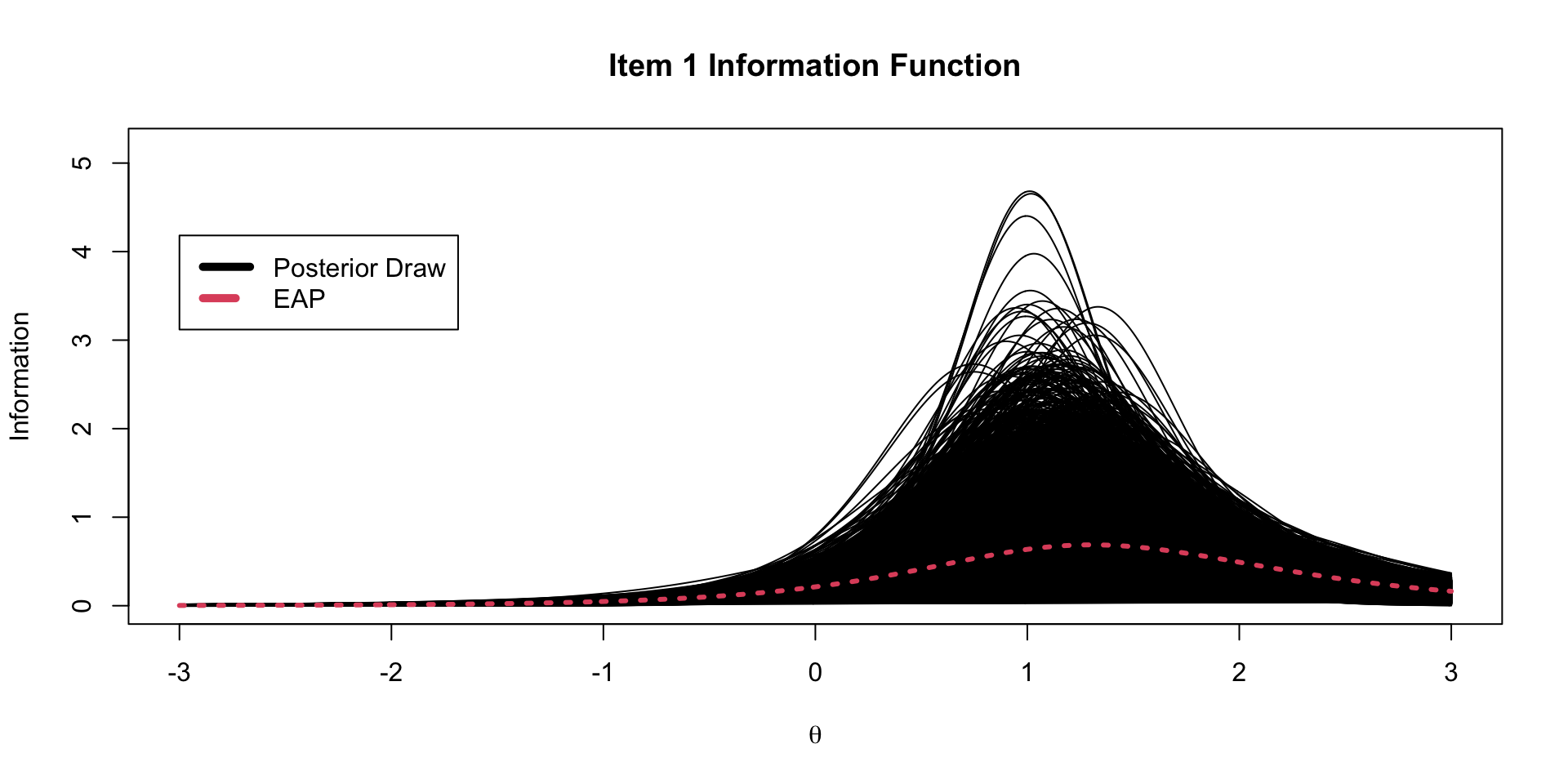
Item Information

An item information function quantifies the amount of information about the latent trait provided by an item

Note: the derivation of information is for MAP estimates (so not the contribution to the posterior standard deviation)

For a given value of \(\theta\), we can calculate an item’s information by taking the second partial derivative the model/data likelihood for an time with respect to \(\theta\)

For the two-parameter logistic model this is:

\[I_i\left( \theta \right) = a_i^2 \left(\frac{\exp \left(a_i \left(\theta -b_i \right) \right)}{1+ \exp \left(a_i \left(\theta-b_i \right) \right)} \right) \left(1-\frac{\exp \left(a_i \left(\theta -b_i \right) \right)}{1+ \exp \left(a_i \left(\theta-b_i \right) \right)} \right)\]

Item Information from Markov Chains

Using generated quantities, we can also calculate the item information for each item at each step of the chain.

We must also use a set of theta values to calculate this across (as with the TCC)

Item Information Functions

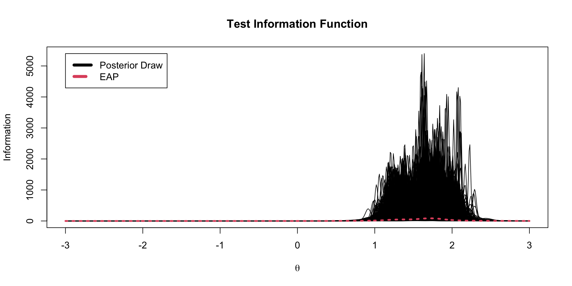
Test Information Function

The test information function is the sum of the item information functions for a given value of \(\theta\)

But, as we are in Bayesian, we must also include the information from the prior distribution of \(\theta\)
- Found by taking the second partial derivative of the pdf of the prior distribution with respect to \(\theta\)
- When \(\theta\) has the standardized factor parameterization, this value is simply -1
We can use Stan’s generated quantities to calculate this, too

For the 2PL model, the test information function is then:

\[TIF\left( \theta \right) = -1+ \sum_{i=1}^I a_i^2 \left(\frac{\exp \left(a_i \left(\theta -b_i \right) \right)}{1+ \exp \left(a_i \left(\theta-b_i \right) \right)} \right) \left(1-\frac{\exp \left(a_i \left(\theta -b_i \right) \right)}{1+ \exp \left(a_i \left(\theta-b_i \right) \right)} \right)\]

TIF Spaghetti Plots

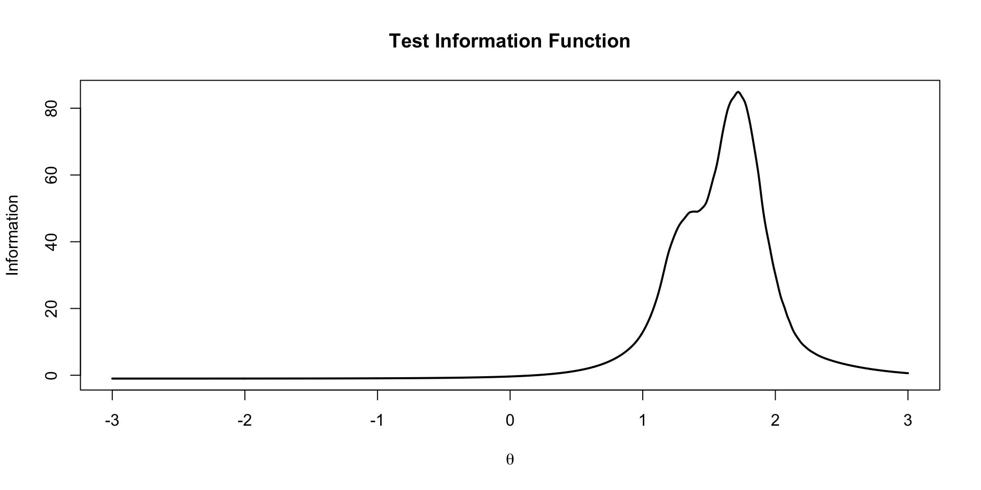
EAP TIF Plot

Other IRT/IFA Models

There are a number of different IRT models that can be implemented in Stan

A slight change is needed in the model statement for the observed data

Up to now, for the 2PL model, we had:

model {
  
  a ~ multi_normal(meanA, covA); // Prior for item discrimination/factor loadings
  b ~ multi_normal(meanB, covB);             // Prior for item intercepts
  
  theta ~ normal(0, 1);                         // Prior for latent variable (with mean/sd specified)
  
  for (item in 1:nItems){
    Y[item] ~ bernoulli_logit(a[item]*(theta - b[item]));
  }

The function bernoulli_logit() will only work for the 1- and 2PL models

It applies the logit link function to the inner portion of the function, then transforms it to a probability, then evaluates the Bernoulli likelihood

Slight Change in Parameterization

To make this more general, we must construct the model using just the Bernoulli function:

model {
  
  a ~ multi_normal(meanA, covA); // Prior for item discrimination/factor loadings
  b ~ multi_normal(meanB, covB);             // Prior for item intercepts
  
  theta ~ normal(0, 1);                         // Prior for latent variable (with mean/sd specified)
  
  for (item in 1:nItems){
    Y[item] ~ bernoulli(inv_logit(a[item]*(theta - b[item])));
  }

Here, the result of inv_logit() is a probability for each person and item

Then, the bernoulli() function calculates the likelihood based on the probability from each item

1PL Model

Item Response Function:

\[ P\left(Y_{pi} = 1 \mid \theta_p \right) = \frac{\exp \left(\theta -b_i \right)}{1+ \exp \left(\theta-b_i \right)} \]

The 1PL model can be built by removing the \(a\) parameter:

data {
  int<lower=0> nObs;                 // number of observations
  int<lower=0> nItems;               // number of items
  array[nItems, nObs] int<lower=0, upper=1>  Y; // item responses in a matrix
  
  vector[nItems] meanB;         // prior mean vector for coefficients
  matrix[nItems, nItems] covB;  // prior covariance matrix for coefficients
}

parameters {
  vector[nObs] theta;                // the latent variables (one for each person)
  vector[nItems] b;             // the factor loadings/item discriminations (one for each item)
}

model {
  b ~ multi_normal(meanB, covB);             // Prior for item intercepts
  theta ~ normal(0, 1);                         // Prior for latent variable (with mean/sd specified)
  
  for (item in 1:nItems){
    Y[item] ~ bernoulli(inv_logit(theta - b[item]));
  }
}

3PL Model

Item Response Function:

\[ P\left(Y_{pi} = 1 \mid \theta_p \right) = c_i +\left(1-c_i\right)\left[\frac{\exp \left(a_i \left(\theta -b_i \right) \right)}{1+ \exp \left(a_i \left(\theta-b_i \right) \right)}\right] \]

parameters {
  vector[nObs] theta;                // the latent variables (one for each person)
  vector[nItems] a;
  vector[nItems] b;             // the factor loadings/item discriminations (one for each item)
  vector<lower=0, upper=1>[nItems] c;
}

model {
  a ~ multi_normal(meanA, covA);             // Prior for item intercepts
  b ~ multi_normal(meanB, covB);             // Prior for item intercepts
  c ~ beta(1,1);                              // Simple prior for c parameter
  
  theta ~ normal(0, 1);                         // Prior for latent variable (with mean/sd specified)
  
  for (item in 1:nItems){
    Y[item] ~ bernoulli(c[item] + (1-c[item])*inv_logit(a[item]*(theta - b[item])));
  }
}

Two-Parameter Normal Ogive Model

Item Response Function:

\[ P\left(Y_{pi} = 1 \mid \theta_p \right) = \Phi \left(a_i \left(\theta -b_i \right)\right) \]

Stan’s function Phi() converts the term in the function to a probability using the inverse normal CDF

Wrapping Up

This lecture covered models for dichotomous data

Many different models can be estimated using Stan with minimal changes to syntax
All IRT auxiliary statistics (i.e, TIF, TCC, IIF) can be computed within Stan

Generalized Measurement Models: Modeling Observed Dichotomous Data

Today’s Lecture Objectives

Example Data: Conspiracy Theories

Please note, the purpose of this survey was to study individual beliefs regarding conspiracies. The questions can provoke some strong emotions given the world we live in currently. All questions were approved by university IRB prior to their use.

Conspiracy Theory Questions 1-5

Conspiracy Theory Questions 6-10

Making Our Data Dichotomous

Examining Dichotomous Data

The Bernoulli Distribution

Definition: Dichotomous vs. Binary

Models with Bernoulli Distributions

Link Functions for Bernoulli Distributions

Less Common Link Functions

Inverse Link Functions

Latent Variable Models with Bernoulli Distributions for Observed Variables

Model Family Names

Differences from Normal Distributions

From Model Scale to Data Scale

Modeling All Data

Measurement Model Analysis Steps

Measurement Model Auxiliary Components

Model Specification

Model (Data) Likelihood Functions

Model (Data) Log Likelihood Functions

Model (Data) Log Likelihood Functions

Model (Data) Log Likelihood Functions for \(\theta_p\)

Model (Data) Log Likelihood Functions

Model (Data) Log Likelihood Functions

Stan’s model Block

Stan’s parameters Block

Stan’s data {} Block

Change to Data List for Stan Import

Running the Model In Stan

Model Results

Modeling Strategy vs. Didactic Strategy

Investigating Item Parameters

Posterior ICC Plots

Investigating the Item Parameters

Investigating the Item Parameters

Investigating the Item Parameters

Investigating the Item Parameters

Investigating the Item Parameters

Investigating the Latent Variables

EAP Estimates of Latent Variables

Density of EAP Estimates

Comparing Two Posterior Distributions

Comparing EAP Estimates with Posterior SDs

Comparing EAP Estimates with Sum Score

Discrimination/Difficulty Parameterization

Comparisons of Parameterizations

Calculating Discrimination/Difficulty Parameters in Generated Quantities

Discrimination/Difficulty Parameter Estimates

Estimating the Discrimination/Difficulty Model

Model Results

Comparing Difficulty Parameters

Comparing Difficulty Parameters: Plot

Comparing Discrimination Parameters

Comparing Discrimination Parameters: Plot

Comparing Theta EAP Estimates

Comparing Theta SD Estimates

Posterior Distributions Are Different

Estimating IRT Model Auxiliary Statistics

Range of \(\theta\)

Test Characteristic Curves

TCC Plots

Item Information

Item Information from Markov Chains

Item Information Functions

Test Information Function

TIF Spaghetti Plots

EAP TIF Plot

Other IRT/IFA Models

Slight Change in Parameterization

1PL Model

3PL Model

Two-Parameter Normal Ogive Model

Wrapping Up

Stan’s `model` Block

Stan’s `parameters` Block

Stan’s `data {}` Block