Generalized Measurement Models: Modeling Multidimensional Latent Variables

Lecture 4e

Today’s Lecture Objectives

Show how to estimate multidimensional latent variable models with polytomous data

Example Data: Conspiracy Theories

Today’s example is from a bootstrap resample of 177 undergraduate students at a large state university in the Midwest. The survey was a measure of 10 questions about their beliefs in various conspiracy theories that were being passed around the internet in the early 2010s. Additionally, gender was included in the survey. All items responses were on a 5- point Likert scale with:

Strongly Disagree
Disagree
Neither Agree or Disagree
Agree
Strongly Agree

Please note, the purpose of this survey was to study individual beliefs regarding conspiracies. The questions can provoke some strong emotions given the world we live in currently. All questions were approved by university IRB prior to their use.

Our purpose in using this instrument is to provide a context that we all may find relevant as many of these conspiracy theories are still prevalent today.

Conspiracy Theory Questions 1-5

Questions:

The U.S. invasion of Iraq was not part of a campaign to fight terrorism, but was driven by oil companies and Jews in the U.S. and Israel.
Certain U.S. government officials planned the attacks of September 11, 2001 because they wanted the United States to go to war in the Middle East.
President Barack Obama was not really born in the United States and does not have an authentic Hawaiian birth certificate.
The current financial crisis was secretly orchestrated by a small group of Wall Street bankers to extend the power of the Federal Reserve and further their control of the world’s economy.
Vapor trails left by aircraft are actually chemical agents deliberately sprayed in a clandestine program directed by government officials.

Conspiracy Theory Questions 6-10

Questions:

Billionaire George Soros is behind a hidden plot to destabilize the American government, take control of the media, and put the world under his control.
The U.S. government is mandating the switch to compact fluorescent light bulbs because such lights make people more obedient and easier to control.
Government officials are covertly Building a 12-lane "NAFTA superhighway" that runs from Mexico to Canada through America’s heartland.
Government officials purposely developed and spread drugs like crack-cocaine and diseases like AIDS in order to destroy the African American community.
God sent Hurricane Katrina to punish America for its sins.

Latent Variables

The Latent Variables

Latent variables are built by specification:

What is their distribution? (nearly all are normally distributed)
How do you specify their scale: mean and standard deviation? (step two in our model analysis steps)

You create latent variables by specifying which items measure which latent variables in an analysis model

Called different names by different fields:
- Alignment (educational measurement)
- Factor pattern matrix (factor analysis)
- Q-matrix (Question matrix; diagnostic models and multidimensional IRT)

From Q-matrix to Model

The alignment provides a specification of which latent variables are measured by which items

Sometimes we say items “load onto” factors

The mathematical definition of either of these terms is simply whether or not a latent variable appears as a predictor for an item

For instance, item one appears to measure nongovernment conspiracies, meaning its alignment (row vector of the Q-matrix) would be:

   Gov NonGov 
     0      1

The model for the first item is then built with only the factors measured by the item as being present:

\[ f(E\left(Y_{p1} \mid \boldsymbol{\theta}_p\right) ) = \mu_1 + \lambda_{11} \theta_{p1} \]

From Q-matrix to Model

The model for the first item is then built with only the factors measured by the item as being present:

\[ f(E\left(Y_{p1} \mid \boldsymbol{\theta}_p\right) ) = \mu_1 + \lambda_{11} \theta_{p1} \]

Where:

\(\mu_1\) is the item intercept
\(\lambda_{11}\) is the factor loading for item 1 (the first subscript) for factor 1 (the second subscript)
\(\theta_{p1}\) is the value of the latent variable for person \(p\) and factor 1

The second factor is not included in the model for the item.

More Q-matrix Stuff

We could show the model with the Q-matrix entries:

\[ f(E\left(Y_{p1} \mid \boldsymbol{\theta}_p\right) ) = \mu_1 + q_{11}\left( \lambda_{11} \theta_{p1} \right) + q_{12}\left( \lambda_{12} \theta_{p2} \right) = \mu_1 + \boldsymbol{\theta}_p \text{diag}\left(\boldsymbol{q}_i \right) \boldsymbol{\lambda}_{1} \]

Where:

\(\boldsymbol{\lambda}_{1} = \left[ \begin{array}{c} \lambda_{11} \\ \lambda_{12} \end{array} \right]\) contains all possible factor loadings for item 1 (size \(2 \times 1\))
\(\boldsymbol{\theta}_p = \left[ \begin{array}{cc} \theta_{p1} & \theta_{p2} \\ \end{array} \right]\) contains the factor scores for person \(p\) (size \(1 \times 2\))
\(\text{diag}\left(\boldsymbol{q}_i \right) = \boldsymbol{q}_i \left[ \begin{array}{cc} 1 & 0 \\ 0 & 1 \end{array} \right] = \left[ \begin{array}{cc} 0 & 1 \\ \end{array} \right] \left[ \begin{array}{cc} 1 & 0 \\ 0 & 1 \end{array} \right] = \left[ \begin{array}{cc} 0 & 0 \\ 0 & 1 \end{array} \right]\) is a diagonal matrix of ones times the vector of Q-matrix entries for item 1

The matrix product then gives:

\[\boldsymbol{\theta}_p \text{diag}\left(\boldsymbol{q}_i \right) \boldsymbol{\lambda}_{1} = \left[ \begin{array}{cc} \theta_{p1} & \theta_{p2} \\ \end{array} \right]\left[ \begin{array}{cc} 0 & 0 \\ 0 & 1 \end{array} \right] \left[ \begin{array}{c} \lambda_{11} \\ \lambda_{12} \end{array} \right] = \left[ \begin{array}{cc} \theta_{p1} & \theta_{p2} \\ \end{array} \right]\left[ \begin{array}{c} 0 \\ \lambda_{12} \end{array} \right] = \lambda_{12}\theta_{p2}\]

The Q-matrix functions like a partial version of the model (predictor) matrix that we saw in linear models

Today’s Q-matrix

       Gov NonGov
item1    0      1
item2    1      0
item3    0      1
item4    0      1
item5    1      0
item6    0      1
item7    1      0
item8    1      0
item9    1      0
item10   0      1

Given the Q-matrix each item has its own model using the alignment specifications

\[ \begin{array}{c} f(E\left(Y_{p1} \mid \boldsymbol{\theta}_p\right) ) = \mu_1 + \lambda_{12} \theta_{p2} \\ f(E\left(Y_{p2} \mid \boldsymbol{\theta}_p\right) ) = \mu_2 + \lambda_{21} \theta_{p1} \\ f(E\left(Y_{p3} \mid \boldsymbol{\theta}_p\right) ) = \mu_3 + \lambda_{32} \theta_{p2} \\ f(E\left(Y_{p4} \mid \boldsymbol{\theta}_p\right) ) = \mu_4 + \lambda_{42} \theta_{p2} \\ f(E\left(Y_{p5} \mid \boldsymbol{\theta}_p\right) ) = \mu_5 + \lambda_{51} \theta_{p1} \\ f(E\left(Y_{p6} \mid \boldsymbol{\theta}_p\right) ) = \mu_6 + \lambda_{62} \theta_{p2} \\ f(E\left(Y_{p7} \mid \boldsymbol{\theta}_p\right) ) = \mu_7 + \lambda_{71} \theta_{p1} \\ f(E\left(Y_{p8} \mid \boldsymbol{\theta}_p\right) ) = \mu_8 + \lambda_{81} \theta_{p1} \\ f(E\left(Y_{p9} \mid \boldsymbol{\theta}_p\right) ) = \mu_9 + \lambda_{91} \theta_{p1} \\ f(E\left(Y_{p,10} \mid \boldsymbol{\theta}_p\right) ) = \mu_{10} + \lambda_{10,2} \theta_{p2} \\ \end{array} \]

Our Example: Multivariate Normal Distribution

For our example, we will assume the set of traits follows a multivariate normal distribution

\[ f\left(\boldsymbol{\theta}_p \right) = \left(2 \pi \right)^{-\frac{D}{2}} \det\left(\boldsymbol{\Sigma}_\theta \right)^{-\frac{1}{2}}\exp\left[-\frac{1}{2}\left(\boldsymbol{\theta}_p - \boldsymbol{\mu}_\theta \right)^T\boldsymbol{\Sigma}_\theta^{-1}\left(\boldsymbol{\theta}_p - \boldsymbol{\mu}_\theta \right) \right] \] Where:

\(\pi \approx 3.14\)
\(D\) is the number of latent variables (dimensions)
\(\boldsymbol{\Sigma}_\theta\) is the covariance matrix of the latent variables
- \(\boldsymbol{\Sigma}_\theta^{-1}\) is the inverse of the covariance matrix
\(\boldsymbol{\mu}_\theta\) is the mean vector of the latent variables
\(\det\left( \cdot\right)\) is the matrix determinant function
\(\left(\cdot \right)^T\) is the matrix transpose operator

Alternatively, we would specify \(\boldsymbol{\theta}_p \sim N_D\left( \boldsymbol{\mu}_\theta, \boldsymbol{\Sigma}_\theta \right)\); but, we cannot always estimate \(\boldsymbol{\mu}_\theta\) and \(\boldsymbol{\Sigma}_\theta\)

Identification of Latent Traits, Part 1

Psychometric models require two types of identification to be valid:

Empirical Identification

The minimum number of items that must measure each latent variable
From CFA: three observed variables for each latent variable (or two if the latent variable is correlated with another latent variable)

Bayesian priors can help to make models with fewer items than these criteria suggest estimable

The parameter estimates (item parameters and latent variable estimates) often have MCMC convergence issues and should not be trusted
Use the CFA standard in your work

Identification of Latent Traits, Part 2

Psychometric models require two types of identification to be valid:

Scale Identification (i.e., what the mean/variance is for each latent variable)

The additional set of constraints needed to set the mean and standard deviation (variance) of the latent variables
Two main methods to set the scale:
- Marker item parameters
  - For variances: Set the loading/slope to one for one observed variable per latent variable
    - Can estimate the latent variable’s variance (the diagonal of \(\boldsymbol{\Sigma}_\theta\))
  - For means: Set the item intercept to one for one observed variable perlatent variable
    - Can estimate the latent variable’s mean (in \(\boldsymbol{\mu}_\theta\))
- Standardized factors
  - Set the variance for all latent variables to one
  - Set the mean for all latent variables to zero
  - Estimate all unique off-diagonal correlations (covariances) in \(\boldsymbol{\Sigma}_\theta\)

Observed Item Model

For each item, we will use a graded- (ordinal logit) response modelwhere:

\[P\left(Y_{ic } = c \mid \theta_p \right) = \left\{ \begin{array}{lr} 1-P\left(Y_{i1} \gt 1 \mid \theta_p \right) & \text{if } c=1 \\ P\left(Y_{i{c-1}} \gt c-1 \mid \theta_p \right) - P\left(Y_{i{c}} \gt c \mid \theta_p \right) & \text{if } 1<c<C_i \\ P\left(Y_{i{C_i -1} } \gt C_i-1 \mid \theta_p \right) - 0 & \text{if } c=C_i \\ \end{array} \right.\]

Where:

\[ P\left(Y_{i{c}} > c \mid \theta \right) = \frac{\exp(\mu_{ic}+\lambda_i\theta_p)}{1+\exp(\mu_{ic}+\lambda_i\theta_p)}\]

With:

\(C_i-1\) Ordered intercepts: \(\mu_1 > \mu_2 > \ldots > \mu_{C_i-1}\)

Building the Multidimensional Model in Stan

Observed Item Model in Stan

As Stan uses thresholds instead of intercepts, our model then becomes:

Where:

\[ P\left(Y_{i{c}} > c \mid \theta \right) = \frac{\exp(-\tau_{ic}+\lambda_i\theta_p)}{1+\exp(-\tau_{ic}+\lambda_i\theta_p)}\]

With:

\(C_i-1\) Ordered thresholds: \(\tau_1 < \tau_2 < \ldots < \tau_{C_i-1}\)

We can convert thresholds to intercepts by multiplying by negative one: \(\mu_c = -\tau_c\)

Stan Model Block

model {
  
  lambda ~ multi_normal(meanLambda, covLambda); 
  thetaCorrL ~ lkj_corr_cholesky(1.0);
  theta ~ multi_normal_cholesky(meanTheta, thetaCorrL);    
  
  
  for (item in 1:nItems){
    thr[item] ~ multi_normal(meanThr[item], covThr[item]);            
    Y[item] ~ ordered_logistic(thetaMatrix*lambdaMatrix[item,1:nFactors]', thr[item]);
  }
  
  
}

Notes:

thetaMatrix is matrix of latent variables for each person \(\boldsymbol{\Theta}\) (size \(N \times D\); \(N\) is number of people, \(D\) is number of dimensions)
lambdaMatrix is, for each item, a matrix of factor loading/discrimination parameters along with zeros by Q-matrix (size \(I \times D\); \(I\) is number of items)
- The transpose of one row of the lambda matrix is used, resulting in a scalar for each person
lambda is a vector of estimated factor loadings (we use a different block to put these into lambdaMatrix)
- Each factor loading has a (univariate) normal distribution for a prior

More Model Block Notes:

model {
  
  lambda ~ multi_normal(meanLambda, covLambda); 
  thetaCorrL ~ lkj_corr_cholesky(1.0);
  theta ~ multi_normal_cholesky(meanTheta, thetaCorrL);    
  
  
  for (item in 1:nItems){
    thr[item] ~ multi_normal(meanThr[item], covThr[item]);            
    Y[item] ~ ordered_logistic(thetaMatrix*lambdaMatrix[item,1:nFactors]', thr[item]);
  }
  
  
}

Notes:

theta is an array of latent variables (we use a different block to put these into thetaMatrix)
theta follows a multivariate normal distribution as a prior where:
- We set all means of theta to zero (the mean for each factor is set to zero)
- We set all variances of theta to one (the variance for each factor is set to one)
- We estimate a correlation matrix of factors \(\textbf{R}_\theta\) using a so-called LKJ prior distribution
  - LKJ priors are found in Stan and make modeling correlations very easy
Of note: we are using the Cholesky forms of the functions lkj_corr_cholesky and multi_normal_cholesky

LKJ Priors for Correlation Matrices

From Stan’s Functions Reference, for a correlation matrix \(\textbf{R}_\theta\)

Correlation Matrix Properties:

Positive definite (determinant greater than zero; \(\det\left(R_\theta \right) >0\)
Symmetric
Diagonal values are all one

LKJ Prior, with hyperparameter \(\eta\), is proportional to the determinant of the correlation matrix

\[\text{LKJ}\left(\textbf{R}_\theta \mid \eta \right) \propto \det\left(\textbf{R}_\theta \right)^{(\eta-1)} \] Where:

Density is uniform over correlation matrices with \(\eta=1\)
With \(\eta>1\), identity matrix is modal (moves correlations toward zero)
With \(0<\eta<1\), density has a trough at the identity (moves correlations away from zero)

For this example, we set \(\eta=1\), noting a uniform prior over all correlation matrices

Cholesky Decomposition

The functions we are using do not use the correlation matrix directly

The problem:

The issue: We need the inverse and determinant to calculate the density of a multivariate normal distribution
- Inverses and determinants are numerically unstable (computationally) in general form

The solution:

Convert \(R_\theta\) to a triangular form using the Cholesky decomposition

\[\textbf{R}_\theta = \textbf{L}_\theta \textbf{L}_\theta^T\]

Cholesky Decomposition Math

\(\det\left(\textbf{R}_\theta \right) = \det\left(\textbf{L}_\theta \textbf{L}_\theta^T\right) = \det\left(\textbf{L}_\theta\right) \det\left(\textbf{L}_\theta^T\right) = \det\left(\textbf{L}_\theta\right)^2 = \left(\prod_{d=1}^D l_{d,d}\right)^2\) (note: product becomes sum for log-likelihood)
For the inverse, we work with the term in the exponent of the MVN pdf:

\[-\frac{1}{2}\left(\boldsymbol{\theta}_p - \boldsymbol{\mu}_\theta \right)^T\textbf{R}_\theta^{-1}\left(\boldsymbol{\theta}_p - \boldsymbol{\mu}_\theta \right) = -\frac{1}{2}\left(\boldsymbol{\theta}_p - \boldsymbol{\mu}_\theta \right)^T\left(\textbf{L}_\theta \textbf{L}_\theta^T\right)^{-1}\left(\boldsymbol{\theta}_p - \boldsymbol{\mu}_\theta \right) \]

\[ -\frac{1}{2}\left(\boldsymbol{\theta}_p - \boldsymbol{\mu}_\theta \right)^T\textbf{L}_\theta^{-T} \textbf{L}_\theta^{-1}\left(\boldsymbol{\theta}_p - \boldsymbol{\mu}_\theta \right)\] Then, we solve by back substitution: \(\left(\boldsymbol{\theta}_p - \boldsymbol{\mu}_\theta \right)^T\textbf{L}_\theta^{-T}\)

We can then multiply this result by itself to form the term in the exponent (times \(-\frac{1}{2}\))
Back substitution involves far fewer steps, minimizing the amount of rounding error in the process of forming the inverse

Most algorithms using MVN distributions use some variant of this process (perhaps with a different factorization method such as QR)

Stan Parameters Block

parameters {
  array[nObs] vector[nFactors] theta;                // the latent variables (one for each person)
  array[nItems] ordered[maxCategory-1] thr; // the item thresholds (one for each item category minus one)
  vector[nLoadings] lambda;             // the factor loadings/item discriminations (one for each item)
  cholesky_factor_corr[nFactors] thetaCorrL;
}

Notes:

theta is an array (for the MVN prior)
thr is the same as the unidimensional model
lambda is the vector of all factor loadings to be estimated (needs nLoadings)
thetaCorrL is of type cholesky_factor_corr, a built in type that identifies this as the lower diagonal of a Cholesky-factorized correlation matrix

We need a couple other blocks to link our parameters to the model

Stan Transformed Data Block

transformed data{
  int<lower=0> nLoadings = 0;                                      // number of loadings in model
  
  for (factor in 1:nFactors){
    nLoadings = nLoadings + sum(Qmatrix[1:nItems, factor]);
  }

  array[nLoadings, 2] int loadingLocation;                     // the row/column positions of each loading
  int loadingNum=1;
  
  for (item in 1:nItems){
    for (factor in 1:nFactors){
      if (Qmatrix[item, factor] == 1){
        loadingLocation[loadingNum, 1] = item;
        loadingLocation[loadingNum, 2] = factor;
        loadingNum = loadingNum + 1;
      }
    }
  }

}

Notes:

The transformed data {} block runs prior to the Markov chain
- We use it to create variables that will stay constant throughout the chain
Here, we count the number of loadings in the Q-matrix nLoadings
- We then process the Q-matrix to tell Stan the row and column position of each loading in the loadingsMatrix used in the model {} block
  - For instance, the loading for item one factor two has row position 1 and column position 2
This syntax works for any Q-matrix (but only has main effects in the model)

Stan Transformed Parameters Block

transformed parameters{
  matrix[nItems, nFactors] lambdaMatrix = rep_matrix(0.0, nItems, nFactors);
  matrix[nObs, nFactors] thetaMatrix;
  
  // build matrix for lambdas to multiply theta matrix
  for (loading in 1:nLoadings){
    lambdaMatrix[loadingLocation[loading,1], loadingLocation[loading,2]] = lambda[loading];
  }
  
  for (factor in 1:nFactors){
    thetaMatrix[,factor] = to_vector(theta[,factor]);
  }
  
}

Notes:

The transformed parameters {} block runs prior to each iteration of the Markov chain
- This means it affects the estimation of each type of parameter
We use it to create:
- thetaMatrix (converting theta from an array to a matrix)
- lambdaMatrix (puts the loadings and zeros from the Q-matrix into correct position)
  - lambdaMatrix initializes at zero (so we just have to add the loadings in the correct position)

Stan Data Block

data {
  
  // data specifications  =============================================================
  int<lower=0> nObs;                            // number of observations
  int<lower=0> nItems;                          // number of items
  int<lower=0> maxCategory;       // number of categories for each item
  
  // input data  =============================================================
  array[nItems, nObs] int<lower=1, upper=5>  Y; // item responses in an array

  // loading specifications  =============================================================
  int<lower=1> nFactors;                                       // number of loadings in the model
  array[nItems, nFactors] int<lower=0, upper=1> Qmatrix;
  
  // prior specifications =============================================================
  array[nItems] vector[maxCategory-1] meanThr;                // prior mean vector for intercept parameters
  array[nItems] matrix[maxCategory-1, maxCategory-1] covThr;  // prior covariance matrix for intercept parameters
  
  vector[nItems] meanLambda;         // prior mean vector for discrimination parameters
  matrix[nItems, nItems] covLambda;  // prior covariance matrix for discrimination parameters
  
  vector[nFactors] meanTheta;
}

Notes:

Changes from unidimensional model:
- meanTheta: Factor means (hyperparameters) are added (but we will set these to zero)
- nFactors: Number of latent variables (needed for Q-matrix)
- Qmatrix: Q-matrix for model

Stan Generated Quantities Block

generated quantities{ 
  array[nItems] vector[maxCategory-1] mu;
  corr_matrix[nFactors] thetaCorr;
   
  for (item in 1:nItems){
    mu[item] = -1*thr[item];
  }
  
  
  thetaCorr = multiply_lower_tri_self_transpose(thetaCorrL);
  
}

Notes:

Converts thresholds to intercepts mu
Creates thetaCorr by multiplying Cholesky-factorized lower triangle with upper triangle
- We will only use the parameters of thetaCorr when looking at model output

Stan Analyses

Estimation in Stan

We run stan the same way we have previously:

modelOrderedLogit_samples = modelOrderedLogit_stan$sample(
  data = modelOrderedLogit_data,
  seed = 191120221,
  chains = 4,
  parallel_chains = 4,
  iter_warmup = 2000,
  iter_sampling = 2000,
  init = function() list(lambda=rnorm(nItems, mean=5, sd=1))
)

Notes:

Smaller chain (model takes a lot longer to run)
Still need to keep loadings positive initially

Analysis Results

[1] 1.080608

# A tibble: 54 × 10
   varia…¹    mean  median      sd     mad       q5    q95  rhat ess_b…² ess_t…³
   <chr>     <dbl>   <dbl>   <dbl>   <dbl>    <dbl>  <dbl> <dbl>   <dbl>   <dbl>
 1 lambda…  2.00    1.99   0.266   0.266     1.59    2.46   1.00  2608.   5005. 
 2 lambda…  2.84    2.82   0.382   0.378     2.25    3.50   1.00  2302.   4728. 
 3 lambda…  2.40    2.38   0.337   0.334     1.88    2.98   1.00  3336.   5197. 
 4 lambda…  2.93    2.91   0.397   0.388     2.31    3.62   1.00  3215.   5114. 
 5 lambda…  4.32    4.28   0.587   0.571     3.42    5.34   1.00  2727.   4328. 
 6 lambda…  4.21    4.19   0.571   0.572     3.33    5.20   1.00  2185.   4053. 
 7 lambda…  2.86    2.84   0.412   0.406     2.22    3.57   1.00  2515.   5597. 
 8 lambda…  4.13    4.09   0.561   0.556     3.28    5.11   1.00  2250.   4791. 
 9 lambda…  2.90    2.88   0.426   0.417     2.24    3.66   1.00  3152.   4106. 
10 lambda…  2.44    2.42   0.427   0.414     1.78    3.18   1.00  4581.   4975. 
11 mu[1,1]  1.87    1.86   0.289   0.293     1.41    2.36   1.00  1431.   3230. 
12 mu[2,1]  0.797   0.793  0.310   0.312     0.296   1.31   1.00   893.   1900. 
13 mu[3,1]  0.0833  0.0835 0.265   0.259    -0.356   0.516  1.00   765.   1468. 
14 mu[4,1]  0.983   0.977  0.329   0.327     0.454   1.53   1.00   860.   1584. 
15 mu[5,1]  1.29    1.28   0.434   0.425     0.601   2.03   1.01   637.   1407. 
16 mu[6,1]  0.945   0.934  0.426   0.414     0.283   1.65   1.01   589.   1248. 
17 mu[7,1] -0.124  -0.128  0.302   0.299    -0.615   0.376  1.00   717.   1116. 
18 mu[8,1]  0.670   0.659  0.407   0.401     0.0164  1.36   1.01   576.   1197. 
19 mu[9,1] -0.0781 -0.0805 0.309   0.305    -0.586   0.430  1.00   751.   1420. 
20 mu[10,… -1.37   -1.36   0.322   0.318    -1.92   -0.871  1.00  1074.   2160. 
21 mu[1,2] -0.222  -0.224  0.238   0.233    -0.617   0.167  1.00   992.   2111. 
22 mu[2,2] -1.54   -1.53   0.325   0.321    -2.09   -1.01   1.00   944.   1969. 
23 mu[3,2] -1.12   -1.12   0.278   0.280    -1.58   -0.666  1.00   819.   1839. 
24 mu[4,2] -1.16   -1.15   0.325   0.320    -1.70   -0.636  1.01   729.   1645. 
25 mu[5,2] -1.97   -1.96   0.452   0.448    -2.74   -1.24   1.00   735.   1352. 
26 mu[6,2] -2.02   -2.00   0.443   0.448    -2.75   -1.31   1.01   742.   1545. 
27 mu[7,2] -1.96   -1.95   0.349   0.349    -2.56   -1.41   1.00  1040.   1597. 
28 mu[8,2] -1.86   -1.84   0.429   0.431    -2.58   -1.16   1.01   691.   1230. 
29 mu[9,2] -1.96   -1.95   0.351   0.346    -2.56   -1.41   1.00  1038.   1978. 
30 mu[10,… -2.61   -2.60   0.380   0.378    -3.29   -2.02   1.00  1471.   3186. 
31 mu[1,3] -2.05   -2.04   0.284   0.279    -2.52   -1.59   1.00  1362.   2534. 
32 mu[2,3] -3.40   -3.39   0.416   0.414    -4.10   -2.74   1.00  1609.   3636. 
33 mu[3,3] -3.69   -3.67   0.424   0.418    -4.42   -3.04   1.00  1918.   5037. 
34 mu[4,3] -3.87   -3.85   0.472   0.458    -4.70   -3.12   1.00  1659.   3528. 
35 mu[5,3] -4.57   -4.55   0.607   0.597    -5.61   -3.63   1.00  1247.   3261. 
36 mu[6,3] -5.64   -5.62   0.684   0.684    -6.78   -4.55   1.00  2317.   4484. 
37 mu[7,3] -4.17   -4.14   0.505   0.506    -5.05   -3.39   1.00  2458.   4976. 
38 mu[8,3] -6.44   -6.40   0.784   0.779    -7.79   -5.22   1.00  3305.   5078. 
39 mu[9,3] -3.26   -3.24   0.430   0.430    -3.99   -2.59   1.00  1380.   3264. 
40 mu[10,… -3.78   -3.76   0.468   0.462    -4.57   -3.05   1.00  2149.   2306. 
41 mu[1,4] -3.99   -3.97   0.470   0.454    -4.80   -3.25   1.00  3417.   5173. 
42 mu[2,4] -4.93   -4.90   0.576   0.571    -5.91   -4.04   1.00  3034.   5066. 
43 mu[3,4] -4.79   -4.76   0.559   0.566    -5.74   -3.91   1.00  3136.   3794. 
44 mu[4,4] -4.78   -4.76   0.565   0.556    -5.78   -3.90   1.00  2148.   5506. 
45 mu[5,4] -6.83   -6.78   0.844   0.829    -8.28   -5.51   1.00  2528.   2677. 
46 mu[6,4] -7.96   -7.92   0.987   0.979    -9.62   -6.40   1.00  4736.   6305. 
47 mu[7,4] -5.72   -5.68   0.701   0.693    -6.97   -4.65   1.00  4510.   5613. 
48 mu[8,4] -8.49   -8.41   1.11    1.13    -10.4    -6.81   1.00  5309.   5788. 
49 mu[9,4] -4.96   -4.93   0.593   0.599    -5.97   -4.06   1.00  2448.   5618. 
50 mu[10,… -4.03   -4.01   0.495   0.491    -4.88   -3.26   1.00  2410.   2494. 
51 thetaC…  1       1      0       0         1       1     NA       NA      NA  
52 thetaC…  0.993   0.994  0.00632 0.00496   0.980   0.999  1.08    44.8    94.9
53 thetaC…  0.993   0.994  0.00632 0.00496   0.980   0.999  1.08    44.8    94.9
54 thetaC…  1       1      0       0         1       1     NA       NA      NA  
# … with abbreviated variable names ¹variable, ²ess_bulk, ³ess_tail

Note:

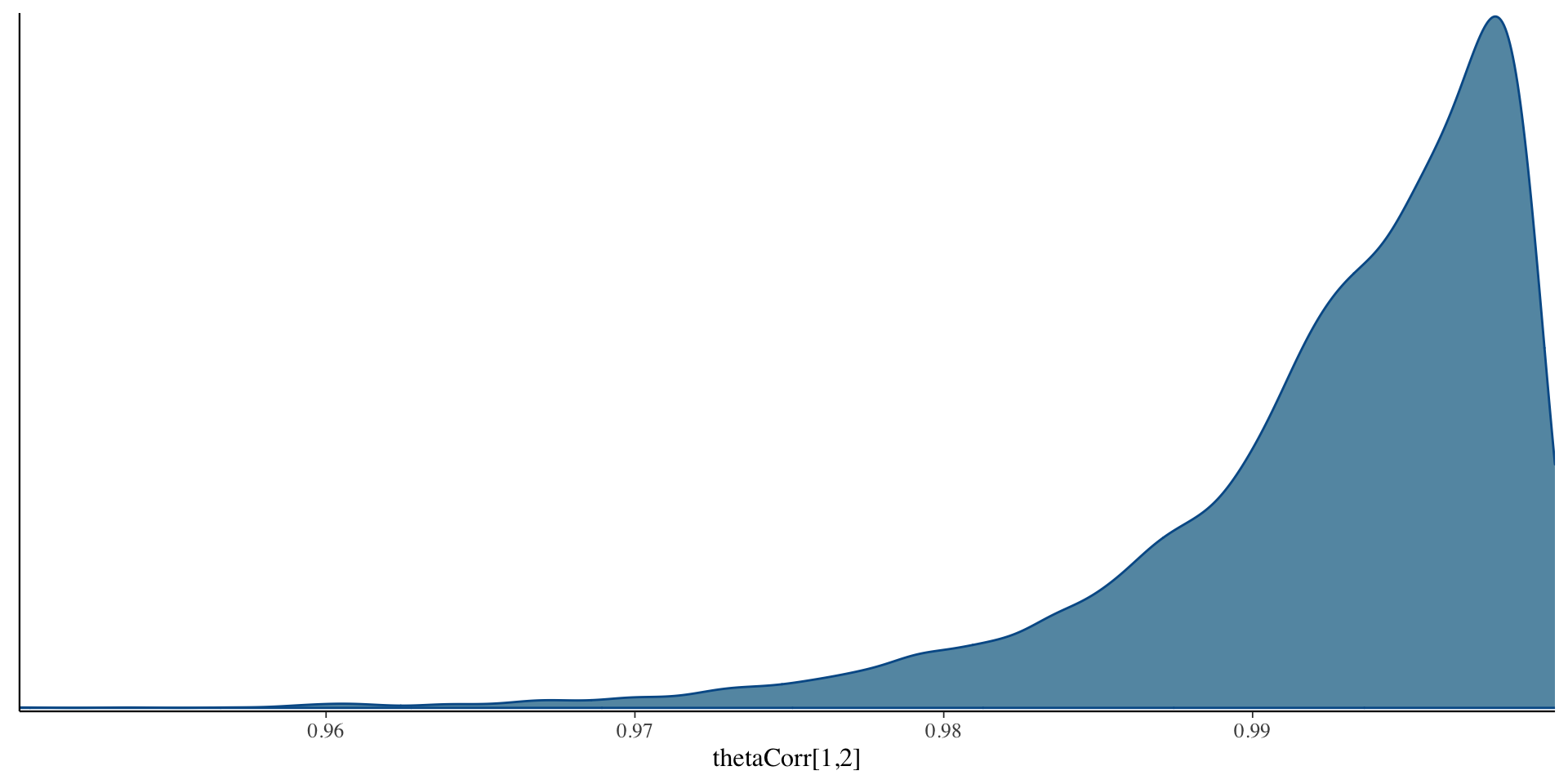
EAP estimate of correlation was 0.993 – indicates only one factor in data

Correlation Chains

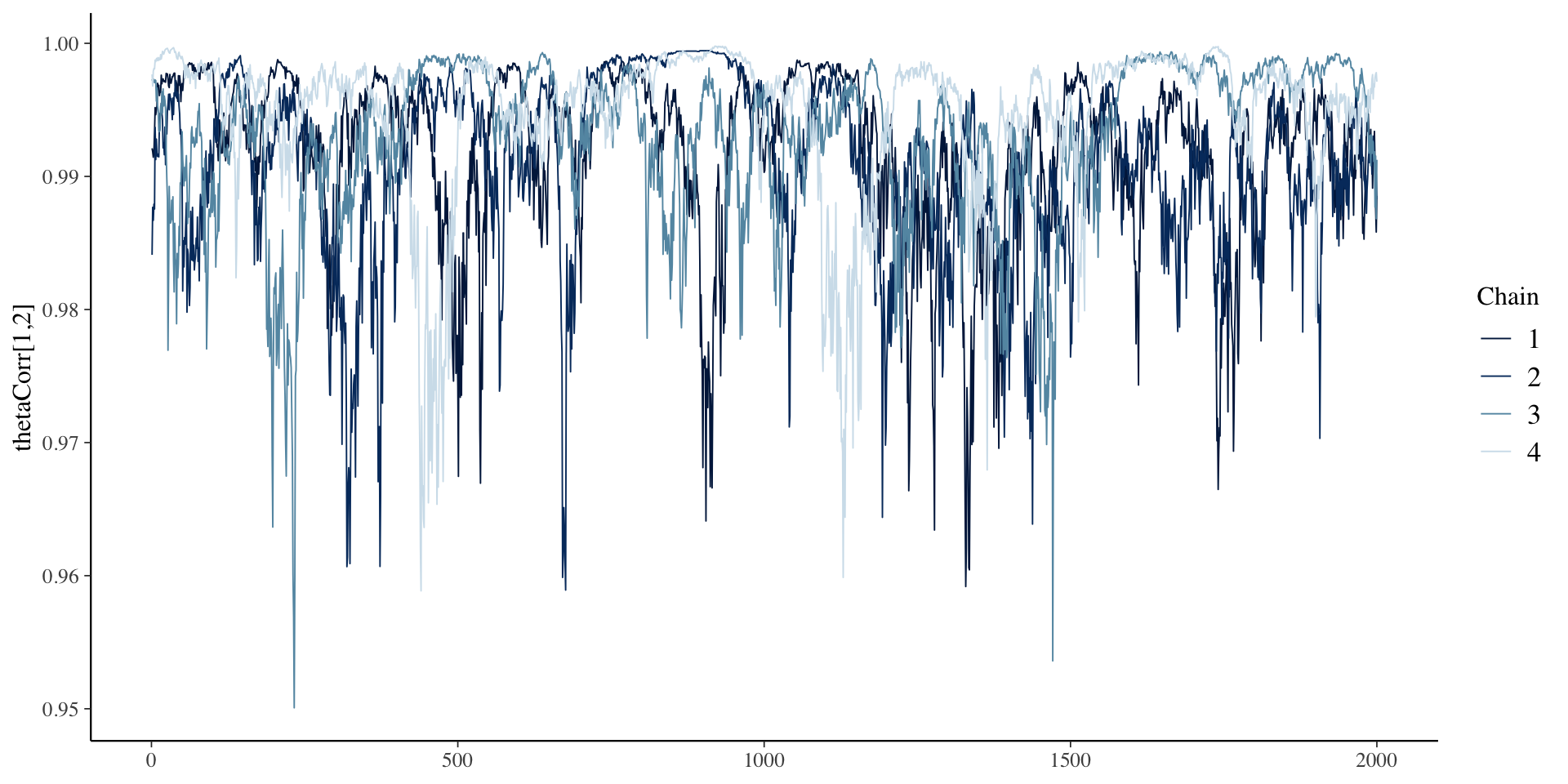
Correlation Posterior Distribution

Example Theta Posterior Distribution

Plots of draws for person 1:

           theta[1,1] theta[1,2]
theta[1,1]  1.0000000  0.8629062
theta[1,2]  0.8629062  1.0000000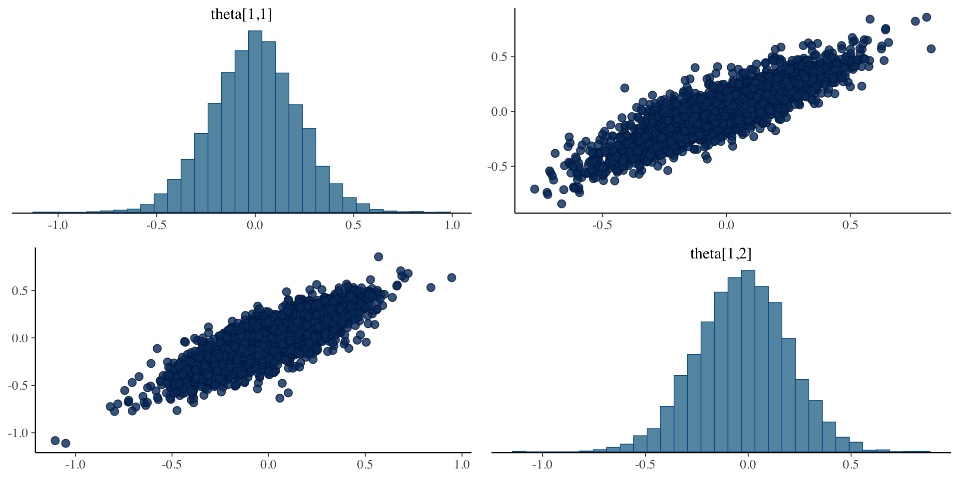

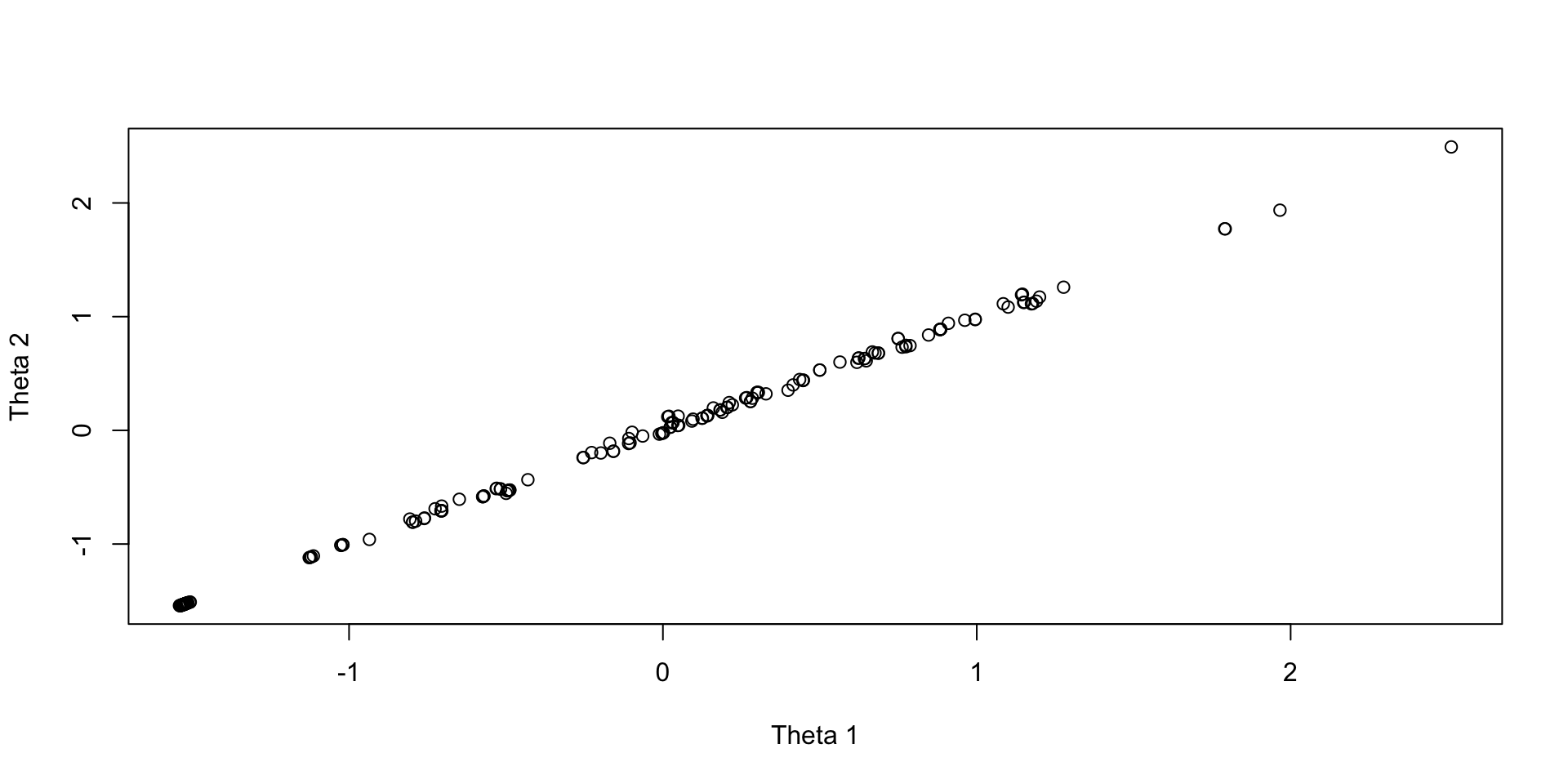
EAP Theta Estimates

Plots of draws for person 1:

Wrapping Up

Stan makes multidimensional latent variable models fairly easy to implement

LKJ prior allows for scale identification with standardized factors
Can use my syntax and import any type of Q-matrix

But…

Estimation is slower (correlations take time)

Generalized Measurement Models: Modeling Multidimensional Latent Variables

Today’s Lecture Objectives

Example Data: Conspiracy Theories

Please note, the purpose of this survey was to study individual beliefs regarding conspiracies. The questions can provoke some strong emotions given the world we live in currently. All questions were approved by university IRB prior to their use.

Conspiracy Theory Questions 1-5

Conspiracy Theory Questions 6-10

The Latent Variables

From Q-matrix to Model

From Q-matrix to Model

More Q-matrix Stuff

Today’s Q-matrix

Our Example: Multivariate Normal Distribution

Identification of Latent Traits, Part 1

Identification of Latent Traits, Part 2

More on Scale Identification

Observed Item Model

Observed Item Model in Stan

Stan Model Block

More Model Block Notes:

LKJ Priors for Correlation Matrices

Cholesky Decomposition

The problem:

The solution:

Cholesky Decomposition Math

Stan Parameters Block

Stan Transformed Data Block

Stan Transformed Parameters Block

Stan Data Block

Stan Generated Quantities Block

Estimation in Stan

Analysis Results

Correlation Chains

Correlation Posterior Distribution

Example Theta Posterior Distribution

EAP Theta Estimates

Wrapping Up