model {

  initLambda ~ multi_normal(meanLambda, covLambda); // Prior for estimated item discrimination/factor loadings
  thetaSD ~ lognormal(thetaSDmean,thetaSDsd);               // Prior for theta standard deviation
  theta ~ normal(0, thetaSD);                       // Prior for latent variable (with sd specified)

  for (item in 1:nItems){
    thr[item] ~ multi_normal(meanThr[item], covThr[item]);             // Prior for item thresholds
    Y[item] ~ ordered_logistic(lambda[item]*theta, thr[item]);         // Item repsonse model (model/data likelihood)
  }


}Latent Variable Scale Identification Methods
Lecture 4h
Today’s Lecture Objectives
- Show how to estimate the standard deviation of the latent variable
Example Data: Conspiracy Theories
Today’s example is from a bootstrap resample of 177 undergraduate students at a large state university in the Midwest. The survey was a measure of 10 questions about their beliefs in various conspiracy theories that were being passed around the internet in the early 2010s. Additionally, gender was included in the survey. All items responses were on a 5- point Likert scale with:
- Strongly Disagree
- Disagree
- Neither Agree or Disagree
- Agree
- Strongly Agree
Please note, the purpose of this survey was to study individual beliefs regarding conspiracies. The questions can provoke some strong emotions given the world we live in currently. All questions were approved by university IRB prior to their use.
Our purpose in using this instrument is to provide a context that we all may find relevant as many of these conspiracy theories are still prevalent today.
Conspiracy Theory Questions 1-5
Questions:
- The U.S. invasion of Iraq was not part of a campaign to fight terrorism, but was driven by oil companies and Jews in the U.S. and Israel.
- Certain U.S. government officials planned the attacks of September 11, 2001 because they wanted the United States to go to war in the Middle East.
- President Barack Obama was not really born in the United States and does not have an authentic Hawaiian birth certificate.
- The current financial crisis was secretly orchestrated by a small group of Wall Street bankers to extend the power of the Federal Reserve and further their control of the world’s economy.
- Vapor trails left by aircraft are actually chemical agents deliberately sprayed in a clandestine program directed by government officials.
Conspiracy Theory Questions 6-10
Questions:
- Billionaire George Soros is behind a hidden plot to destabilize the American government, take control of the media, and put the world under his control.
- The U.S. government is mandating the switch to compact fluorescent light bulbs because such lights make people more obedient and easier to control.
- Government officials are covertly Building a 12-lane "NAFTA superhighway" that runs from Mexico to Canada through America’s heartland.
- Government officials purposely developed and spread drugs like crack-cocaine and diseases like AIDS in order to destroy the African American community.
- God sent Hurricane Katrina to punish America for its sins.
Model Setup Today
Today, we will revert back to the graded response model assumptions to discuss how to estimate the latent variable standard deviation
\[P\left(Y_{ic } = c \mid \theta_p \right) = \left\{ \begin{array}{lr} 1-P\left(Y_{i1} \gt 1 \mid \theta_p \right) & \text{if } c=1 \\ P\left(Y_{i{c-1}} \gt c-1 \mid \theta_p \right) - P\left(Y_{i{c}} \gt c \mid \theta_p \right) & \text{if } 1<c<C_i \\ P\left(Y_{i{C_i -1} } \gt C_i-1 \mid \theta_p \right) & \text{if } c=C_i \\ \end{array} \right.\]
Where:
\[ P\left(Y_{i{c}} > c \mid \theta \right) = \frac{\exp(-\tau_{ic}+\lambda_i\theta_p)}{1+\exp(-\tau_{ic}+\lambda_i\theta_p)}\]
With:
- \(C_i-1\) Ordered thresholds: \(\tau_1 < \tau_2 < \ldots < \tau_{C_i-1}\)
We can convert thresholds to intercepts by multiplying by negative one: \(\mu_c = -\tau_c\)
Scale Identification Methods
Identification of Latent Traits, Part 1
Psychometric models require two types of identification to be valid:
- Empirical Identification
- The minimum number of items that must measure each latent variable
- From CFA: three observed variables for each latent variable (or two if the latent variable is correlated with another latent variable)
Bayesian priors can help to make models with fewer items than these criteria suggest estimable
- The parameter estimates (item parameters and latent variable estimates) often have MCMC convergence issues and should not be trusted
- Use the CFA standard in your work
Identification of Latent Traits, Part 2
Psychometric models require two types of identification to be valid:
- Scale Identification (i.e., what the mean/variance is for each latent variable)
- The additional set of constraints needed to set the mean and standard deviation (variance) of the latent variables
- Two main methods to set the scale:
- Marker item parameters
- For variances: Set the loading/slope to one for one observed variable per latent variable
- Can estimate the latent variable’s variance (the diagonal of \(\boldsymbol{\Sigma}_\theta\))
- For means: Set the item intercept to one for one observed variable perlatent variable
- Can estimate the latent variable’s mean (in \(\boldsymbol{\mu}_\theta\))
- For variances: Set the loading/slope to one for one observed variable per latent variable
- Standardized factors
- Set the variance for all latent variables to one
- Set the mean for all latent variables to zero
- Estimate all unique off-diagonal correlations (covariances) in \(\boldsymbol{\Sigma}_\theta\)
- Marker item parameters
Marker Items for \(\theta\) Standard Deviations
To estimate the standard deviation of \(\theta\) (a type of empirical prior) * Set one loading/discrimination parameter to one
To estimate the mean of \(\theta\): * Set one threshold parameter to zero * A bit more difficult to implement in Stan * Skipped for today
Under both of these cases, the model/data likelihood is identified * This provides what I call “strong identification” of the posterior distribution
I begin with a single \(\theta\) as it is easier to show * Multidimensional \(\Theta\) comes after
Stan’s Model Block
Notes:
- Here, we are only estimating the standard deviation of \(\theta\)
- We will leave the mean at zero
- We will use a log normal distribution for the SD (needs a mean and SD for hyperparameters)
lambda`` inordered_logistic()function is different frominitLambda```- We need a
transformed parametersblock to set one loading to one
- We need a
Stan’s Parameters Block
parameters {
  vector[nObs] theta;                // the latent variables (one for each person)
  real<lower=0> thetaSD;

  array[nItems] ordered[maxCategory-1] thr; // the item thresholds (one for each item category minus one)
  vector[nItems-1] initLambda;             // the estimated factor loadings (number of items-1 for one marker item)
}
Notes:
thetaSDhas lower bound of zeroinitLambdais lengthnItems-1(one less as we set that one to one)
Stan’s Transformed Parameters Block
Notes:
- We set the first loading to one
- All others are estimated
- Technically, any loading can be set to one
- All are equivalent models based on likelihood
- If an item has very little relation to the latent variable, setting that item’s loading to one can cause estimation problems
- Difficult to tell which item may have problems before the analysis
Stan’s Data Block
data {
  int<lower=0> nObs;                            // number of observations
  int<lower=0> nItems;                          // number of items
  int<lower=0> maxCategory;                     // maximum category across all items

  array[nItems, nObs] int<lower=1, upper=5>  Y; // item responses in an array

  array[nItems] vector[maxCategory-1] meanThr;                    // prior mean vector for intercept parameters
  array[nItems] matrix[maxCategory-1, maxCategory-1] covThr;      // prior covariance matrix for intercept parameters

  vector[nItems-1] meanLambda;         // prior mean vector for discrimination parameters
  matrix[nItems-1, nItems-1] covLambda;  // prior covariance matrix for discrimination parameters

  real thetaSDmean;  // prior mean hyperparameter for theta standard deviation (log normal distribution)
  real thetaSDsd; // prior sd hyperparameter for theta standard deviation (log normal distribution)
}
Notes:
- Here, we need to set mean/sd hyperparameters for the standard deviation of \(\theta\)
R Data List
Notes:
Hyperparameter for location (\(\mu\)) of lognormal distribution is 0
Hyperparameter for scale (\(\sigma\)) of lognormal distribution is 2
Lognormal mean is:
\[\exp \left(\mu +\frac{\sigma^2}{2} \right) = 7.39 \]
- Lognormal SD is:
\[ \sqrt{ \left[ \exp \left( \sigma^2 \right) -1 \right] \exp \left(2\mu + \sigma^2 \right) } = 54.1 \]
Stan Results
[1] 1.004561# A tibble: 51 × 10
variable mean median sd mad q5 q95 rhat ess_bulk
<chr> <dbl> <dbl> <dbl> <dbl> <dbl> <dbl> <dbl> <dbl>
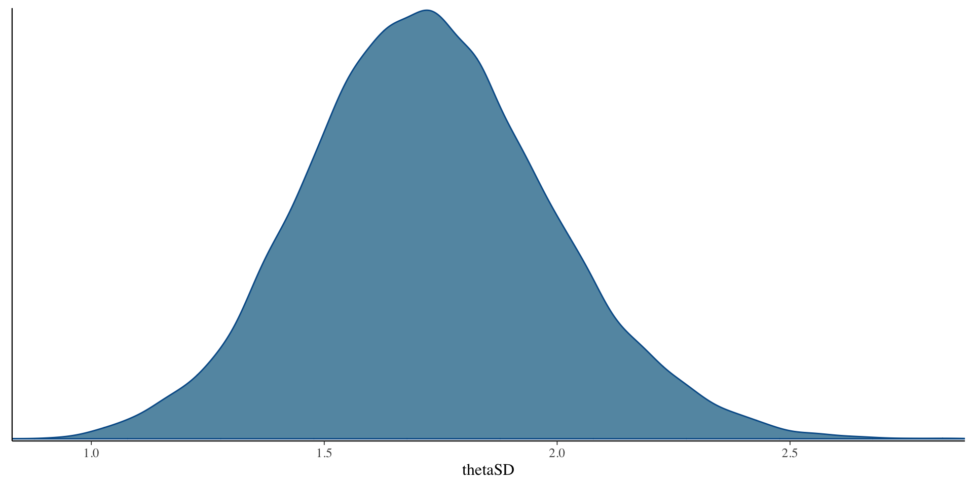
1 thetaSD 1.73 1.72 0.263 0.258 1.31 2.18 1.00 668.
2 lambda[1] 1 1 0 0 1 1 NA NA
3 lambda[2] 1.72 1.68 0.315 0.296 1.26 2.28 1.00 1022.
4 lambda[3] 1.48 1.45 0.303 0.286 1.05 2.03 1.00 969.
5 lambda[4] 1.75 1.72 0.328 0.314 1.28 2.34 1.00 957.
6 lambda[5] 2.82 2.75 0.561 0.529 2.03 3.82 1.00 1002.
7 lambda[6] 2.85 2.79 0.571 0.535 2.04 3.88 1.00 939.
8 lambda[7] 1.84 1.79 0.378 0.349 1.30 2.53 1.00 967.
9 lambda[8] 3.02 2.93 0.628 0.587 2.14 4.15 1.00 1033.
10 lambda[9] 1.78 1.74 0.360 0.335 1.26 2.43 1.00 1027.
11 lambda[10] 1.52 1.48 0.341 0.323 1.03 2.14 1.00 1243.
12 mu[1,1] 1.40 1.39 0.256 0.256 0.987 1.83 1.00 4432.
13 mu[2,1] 0.213 0.216 0.317 0.310 -0.310 0.731 1.00 2901.
14 mu[3,1] -0.428 -0.421 0.293 0.290 -0.922 0.0386 1.00 3460.
15 mu[4,1] 0.378 0.378 0.326 0.318 -0.162 0.910 1.00 3088.
16 mu[5,1] 0.391 0.392 0.476 0.460 -0.394 1.18 1.00 2359.
17 mu[6,1] 0.0218 0.0260 0.481 0.467 -0.780 0.799 1.00 2484.
18 mu[7,1] -0.782 -0.769 0.349 0.341 -1.37 -0.228 1.00 2927.
19 mu[8,1] -0.313 -0.294 0.513 0.499 -1.18 0.490 1.00 2353.
20 mu[9,1] -0.708 -0.699 0.343 0.334 -1.29 -0.168 1.00 3026.
21 mu[10,1] -1.96 -1.93 0.387 0.381 -2.63 -1.36 1.00 4827.
22 mu[1,2] -0.557 -0.554 0.231 0.226 -0.944 -0.184 1.00 2516.
23 mu[2,2] -2.16 -2.15 0.377 0.369 -2.81 -1.57 1.00 3884.
24 mu[3,2] -1.66 -1.65 0.324 0.324 -2.21 -1.15 1.00 4102.
25 mu[4,2] -1.76 -1.75 0.358 0.356 -2.37 -1.20 1.00 3504.
26 mu[5,2] -3.12 -3.09 0.607 0.595 -4.17 -2.20 1.00 3407.
27 mu[6,2] -3.20 -3.16 0.595 0.575 -4.25 -2.30 1.00 3566.
28 mu[7,2] -2.70 -2.68 0.427 0.420 -3.44 -2.04 1.00 4187.
29 mu[8,2] -3.20 -3.16 0.634 0.629 -4.31 -2.25 1.00 3378.
30 mu[9,2] -2.64 -2.61 0.425 0.418 -3.38 -1.97 1.00 4357.
31 mu[10,2] -3.24 -3.21 0.459 0.451 -4.04 -2.54 1.00 6382.
32 mu[1,3] -2.30 -2.29 0.292 0.288 -2.80 -1.84 1.00 1626.
33 mu[2,3] -4.08 -4.06 0.484 0.479 -4.91 -3.32 1.00 5592.
34 mu[3,3] -4.36 -4.33 0.509 0.508 -5.24 -3.57 1.00 8283.
35 mu[4,3] -4.56 -4.53 0.526 0.524 -5.46 -3.74 1.00 7005.
36 mu[5,3] -5.97 -5.91 0.840 0.823 -7.43 -4.70 1.00 5392.
37 mu[6,3] -7.43 -7.34 0.997 0.970 -9.20 -5.94 1.00 7548.
38 mu[7,3] -5.09 -5.06 0.632 0.626 -6.18 -4.11 1.00 7356.
39 mu[8,3] -8.95 -8.84 1.30 1.27 -11.3 -7.03 1.00 8882.
40 mu[9,3] -3.97 -3.94 0.510 0.501 -4.86 -3.18 1.00 5870.
41 mu[10,3] -4.47 -4.44 0.562 0.552 -5.45 -3.60 1.00 8536.
42 mu[1,4] -4.24 -4.21 0.476 0.471 -5.06 -3.50 1.00 2416.
43 mu[2,4] -5.68 -5.66 0.654 0.649 -6.82 -4.67 1.00 9069.
44 mu[3,4] -5.54 -5.50 0.656 0.654 -6.67 -4.52 1.00 11569.
45 mu[4,4] -5.52 -5.49 0.617 0.616 -6.58 -4.56 1.00 8879.
46 mu[5,4] -8.53 -8.44 1.15 1.11 -10.6 -6.81 1.00 8679.
47 mu[6,4] -10.4 -10.3 1.43 1.42 -12.9 -8.26 1.00 11443.
48 mu[7,4] -6.86 -6.81 0.866 0.865 -8.35 -5.52 1.00 10947.
49 mu[8,4] -12.0 -11.8 1.90 1.85 -15.4 -9.18 1.00 12431.
50 mu[9,4] -5.76 -5.71 0.699 0.688 -6.96 -4.67 1.00 9320.
51 mu[10,4] -4.74 -4.70 0.591 0.584 -5.77 -3.83 1.00 9196.
# … with 1 more variable: ess_tail <dbl>SD \(\theta\) Results
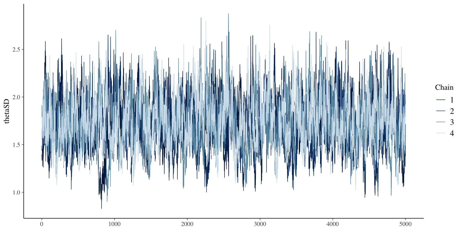
SD \(\theta\) Results
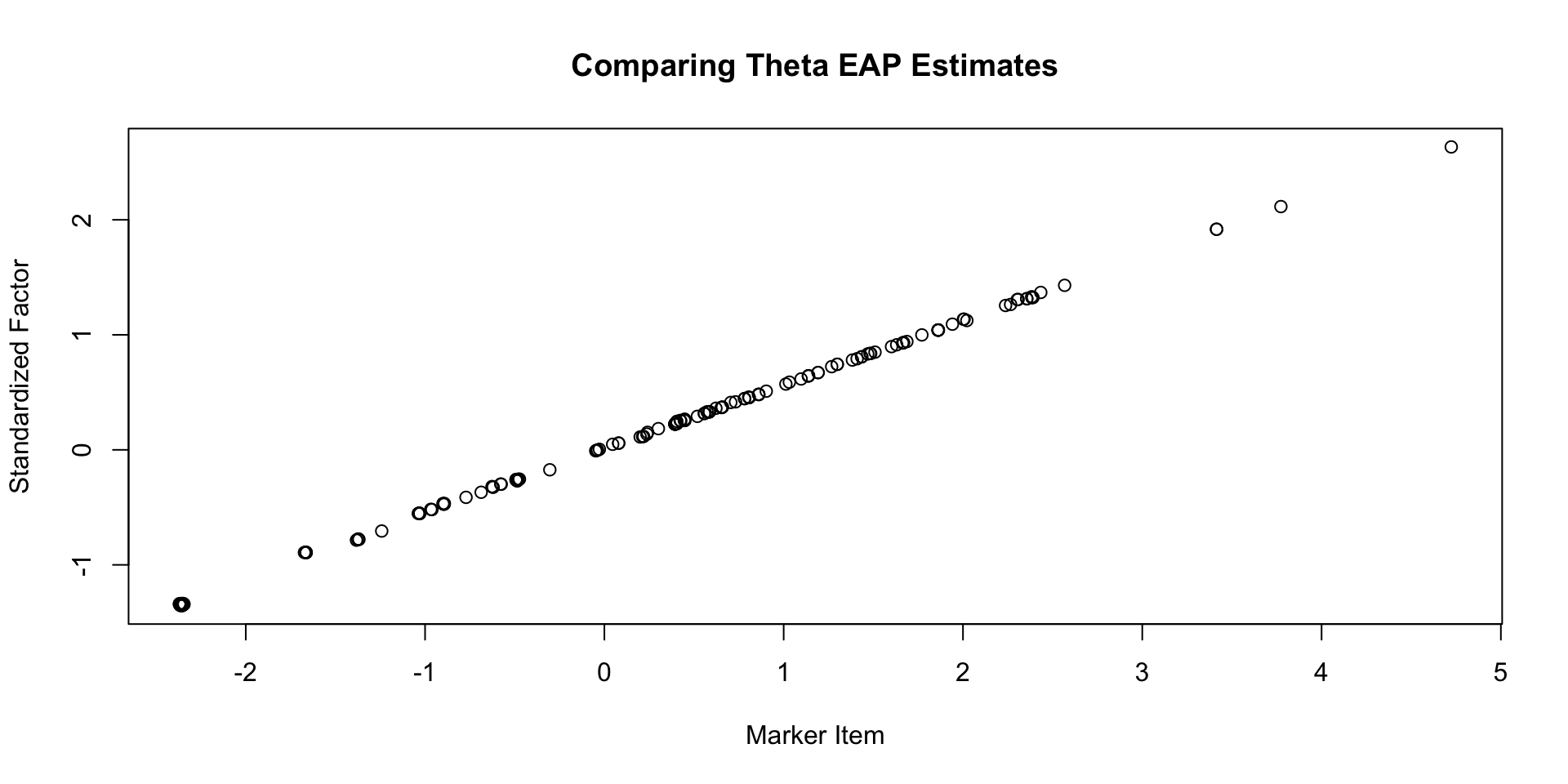
Comparing \(\theta\) EAP Estimates
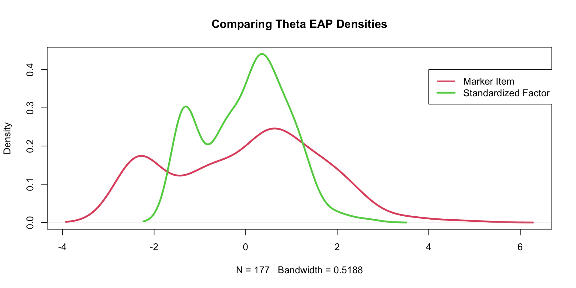
Comparing \(\theta\) EAP Estimates
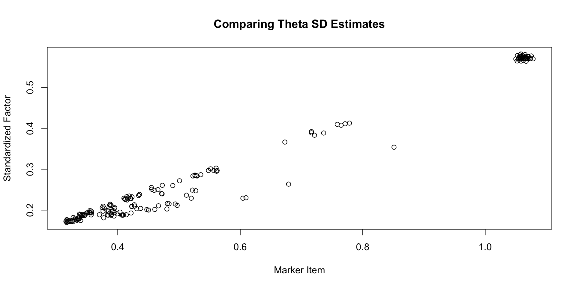
Comparing \(\theta\) SD Estimates
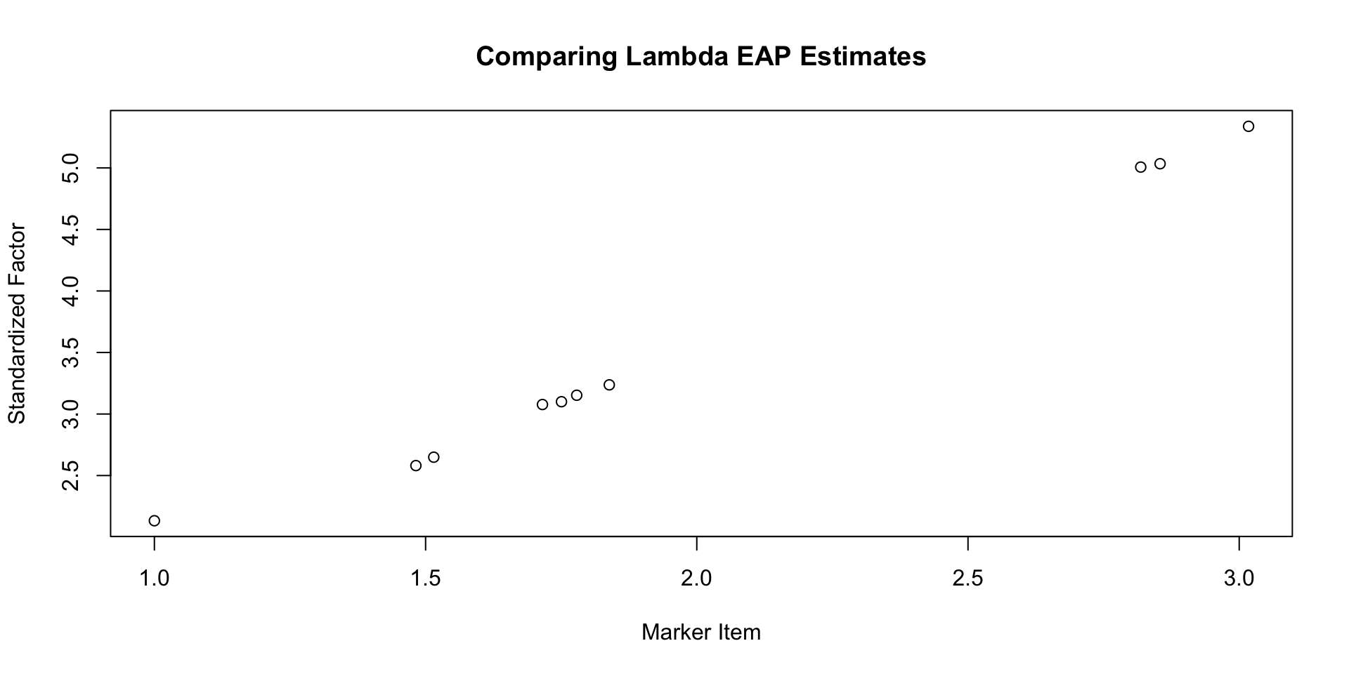
Comparing \(\lambda\) EAP Estimates
Marker Items for Multidimensional Models
Marker Items for Multidimensional Models
We can also build marker items into multidimensional models
- A bit more tricky–we need to estimate the covariance matrix of \(\theta\) now (\(\Sigma_\theta\))
- We accomplish this by pre- and post-multiplying the correlation matrix of \(\theta\) by a diagonal matrix of the standard deviations of \(\theta\)
Stan’s Model Block
model {

  matrix[nFactors, nFactors] thetaCovL;
  initLambda ~ multi_normal(meanLambda, covLambda);

  thetaCorrL ~ lkj_corr_cholesky(1.0);
  thetaSD ~ lognormal(sdThetaLocation,sdThetaScale);

  thetaCovL = diag_pre_multiply(thetaSD, thetaCorrL);
  theta ~ multi_normal_cholesky(meanTheta, thetaCovL);


  for (item in 1:nItems){
    thr[item] ~ multi_normal(meanThr[item], covThr[item]);
    Y[item] ~ ordered_logistic(thetaMatrix*lambdaMatrix[item,1:nFactors]', thr[item]);
  }


}
Notes:
- The
multi_normal_choleskyfunction now uses the covariance matrix - We calculate the covariance matrix using the
thetaCovL = diag_pre_multiply(thetaSD, thetaCorrL);;line - The SDs have a lognormal prior distribution for each
Stan’s Parameters Block
parameters {
  array[nObs] vector[nFactors] theta;                // the latent variables (one for each person)
  array[nItems] ordered[maxCategory-1] thr; // the item thresholds (one for each item category minus one)
  vector[nLoadings-nFactors] initLambda;             // the factor loadings/item discriminations (one for each item)

  cholesky_factor_corr[nFactors] thetaCorrL;
  vector<lower=0>[nFactors] thetaSD;
}
Notes:
- We still have a correlation matrix estimated
- Now adding a vector of SDs
Stan’s Transformed Data Block
transformed data{
  int<lower=0> nLoadings = 0;                                      // number of loadings in model
  array[nFactors] int<lower=0> markerItem = rep_array(0, nFactors);

  for (factor in 1:nFactors){
    nLoadings = nLoadings + sum(Qmatrix[1:nItems, factor]);
  }

  array[nLoadings, 4] int loadingLocation;                     // the row/column positions of each loading, plus marker switch

  int loadingNum=1;
  int lambdaNum=1;
  for (item in 1:nItems){
    for (factor in 1:nFactors){
      if (Qmatrix[item, factor] == 1){
        loadingLocation[loadingNum, 1] = item;
        loadingLocation[loadingNum, 2] = factor;
        if (markerItem[factor] == 0){
          loadingLocation[loadingNum, 3] = 1;     // ==1 if marker item, ==0 otherwise
          loadingLocation[loadingNum, 4] = 0;     // ==0 if not one of estimated lambdas
          markerItem[factor] = item;
        } else {
          loadingLocation[loadingNum, 3] = 0;
          loadingLocation[loadingNum, 4] = lambdaNum;
          lambdaNum = lambdaNum + 1;
        }
        loadingNum = loadingNum + 1;
      }
    }
  }


}
Stan’s Transformed Data Block Notes
- Loading location now lists two additional columns
- An indicator of whether or not to set value to one
- An indicator of which loading in the loading vector is needed if loading is being estimated
Stan’s Transformed Parameters Block
transformed parameters{
  matrix[nItems, nFactors] lambdaMatrix = rep_matrix(0.0, nItems, nFactors);
  matrix[nObs, nFactors] thetaMatrix;

  // build matrix for lambdas to multiply theta matrix

  for (loading in 1:nLoadings){
    if (loadingLocation[loading,3] == 1){
      lambdaMatrix[loadingLocation[loading,1], loadingLocation[loading,2]] = 1.0;
    } else {
      lambdaMatrix[loadingLocation[loading,1], loadingLocation[loading,2]] = initLambda[loadingLocation[loading,4]];
    }
  }

  for (factor in 1:nFactors){
    thetaMatrix[,factor] = to_vector(theta[,factor]);
  }

}
Notes:
- Here, we set the first item’s loading to one for each dimension
- We determine the location of each loading using the results from the transformed data block sorting the Q-matrix
Stan’s Generated Quantities Block
generated quantities{
  array[nItems] vector[maxCategory-1] mu;
  corr_matrix[nFactors] thetaCorr;
  cholesky_factor_cov[nFactors] thetaCov_pre;
  cov_matrix[nFactors] thetaCov;

  for (item in 1:nItems){
    mu[item] = -1*thr[item];
  }

  thetaCorr = multiply_lower_tri_self_transpose(thetaCorrL);
  thetaCov_pre = diag_pre_multiply(thetaSD, thetaCorrL);
  thetaCov = multiply_lower_tri_self_transpose(thetaCov_pre);
}
Notes:
- Now we calculate the covariance matrix here, too
Stan’s Data Block
data {

  // data specifications  =============================================================
  int<lower=0> nObs;                            // number of observations
  int<lower=0> nItems;                          // number of items
  int<lower=0> maxCategory;                     // number of categories for each item

  // input data  =============================================================
  array[nItems, nObs] int<lower=1, upper=5>  Y; // item responses in an array

  // loading specifications  =============================================================
  int<lower=1> nFactors;                                       // number of loadings in the model
  array[nItems, nFactors] int<lower=0, upper=1> Qmatrix;

  // prior specifications =============================================================
  array[nItems] vector[maxCategory-1] meanThr;                // prior mean vector for intercept parameters
  array[nItems] matrix[maxCategory-1, maxCategory-1] covThr;  // prior covariance matrix for intercept parameters

  vector[nItems-nFactors] meanLambda;         // prior mean vector for discrimination parameters
  matrix[nItems-nFactors, nItems-nFactors] covLambda;  // prior covariance matrix for discrimination parameters

  vector[nFactors] meanTheta;
  vector[nFactors] sdThetaLocation;
  vector[nFactors] sdThetaScale;
}
Notes:
- Adding hyperparameters for the SDs of \(theta\)
- No other differences from previous multidimensional model code
R Data List
thetaMean = rep(0, nFactors)
sdThetaLocation = rep(0, nFactors)
sdThetaScale = rep(.5, nFactors)

modelMultidimensionalGRM_markerItem_data = list(
  nObs = nObs,
  nItems = nItems,
  maxCategory = maxCategory,
  Y = t(conspiracyItems),
  nFactors = nFactors,
  Qmatrix = Qmatrix,
  meanThr = thrMeanMatrix,
  covThr = thrCovArray,
  meanLambda = lambdaMeanVecHP,
  covLambda = lambdaCovarianceMatrixHP,
  meanTheta = thetaMean,
  sdThetaLocation = sdThetaLocation,
  sdThetaScale = sdThetaScale
)
Stan Results
 # checking convergence
max(modelMultidimensionalGRM_markerItem_samples$summary()$rhat, na.rm = TRUE)
[1] 1.080386# parameter results
print(modelMultidimensionalGRM_markerItem_samples$summary(variables = c("thetaSD", "thetaCov", "thetaCorr", "lambdaMatrix", "mu")) ,n=Inf)# A tibble: 70 × 10
variable mean median sd mad q5 q95 rhat ess_bulk
<chr> <dbl> <dbl> <dbl> <dbl> <dbl> <dbl> <dbl> <dbl>
1 thetaSD[1] 2.44 2.42 0.345 0.354 1.93 3.02 1.01 296.
2 thetaSD[2] 1.75 1.74 0.247 0.250 1.36 2.17 1.00 505.
3 thetaCov[1,… 6.07 5.87 1.72 1.72 3.71 9.13 1.01 296.
4 thetaCov[2,… 4.23 4.13 0.925 0.864 2.89 5.93 1.00 513.
5 thetaCov[1,… 4.23 4.13 0.925 0.864 2.89 5.93 1.00 513.
6 thetaCov[2,… 3.11 3.02 0.882 0.855 1.85 4.71 1.00 505.
7 thetaCorr[1… 1 1 0 0 1 1 NA NA
8 thetaCorr[2… 0.989 0.992 0.00973 0.00778 0.969 0.999 1.07 41.5
9 thetaCorr[1… 0.989 0.992 0.00973 0.00778 0.969 0.999 1.07 41.5
10 thetaCorr[2… 1 1 0 0 1 1 NA NA
11 lambdaMatri… 0 0 0 0 0 0 NA NA
12 lambdaMatri… 1 1 0 0 1 1 NA NA
13 lambdaMatri… 0 0 0 0 0 0 NA NA
14 lambdaMatri… 0 0 0 0 0 0 NA NA
15 lambdaMatri… 1.96 1.91 0.380 0.348 1.43 2.64 1.01 828.
16 lambdaMatri… 0 0 0 0 0 0 NA NA
17 lambdaMatri… 1.27 1.25 0.245 0.241 0.914 1.70 1.01 401.
18 lambdaMatri… 2.11 2.07 0.434 0.392 1.50 2.90 1.00 900.
19 lambdaMatri… 1.23 1.21 0.228 0.223 0.895 1.62 1.01 489.
20 lambdaMatri… 0 0 0 0 0 0 NA NA
21 lambdaMatri… 1 1 0 0 1 1 NA NA
22 lambdaMatri… 0 0 0 0 0 0 NA NA
23 lambdaMatri… 1.46 1.44 0.278 0.262 1.05 1.95 1.00 768.
24 lambdaMatri… 1.71 1.69 0.304 0.311 1.27 2.24 1.00 669.
25 lambdaMatri… 0 0 0 0 0 0 NA NA
26 lambdaMatri… 2.85 2.80 0.580 0.531 2.04 3.87 1.00 775.
27 lambdaMatri… 0 0 0 0 0 0 NA NA
28 lambdaMatri… 0 0 0 0 0 0 NA NA
29 lambdaMatri… 0 0 0 0 0 0 NA NA
30 lambdaMatri… 1.48 1.44 0.317 0.296 1.02 2.06 1.00 899.
31 mu[1,1] 1.42 1.42 0.259 0.267 0.996 1.85 1.00 767.
32 mu[2,1] 0.248 0.254 0.282 0.280 -0.227 0.702 1.00 742.
33 mu[3,1] -0.442 -0.430 0.293 0.305 -0.941 0.0165 1.00 798.
34 mu[4,1] 0.379 0.375 0.320 0.316 -0.147 0.908 1.00 739.
35 mu[5,1] 0.397 0.412 0.456 0.432 -0.365 1.14 1.01 643.
36 mu[6,1] 0.0324 0.0238 0.482 0.473 -0.754 0.819 1.01 684.
37 mu[7,1] -0.776 -0.755 0.349 0.354 -1.39 -0.237 1.00 658.
38 mu[8,1] -0.285 -0.258 0.509 0.485 -1.15 0.483 1.00 501.
39 mu[9,1] -0.700 -0.701 0.343 0.341 -1.27 -0.173 1.01 453.
40 mu[10,1] -1.99 -1.96 0.388 0.360 -2.69 -1.41 1.00 1338.
41 mu[1,2] -0.571 -0.561 0.235 0.229 -0.961 -0.200 1.00 674.
42 mu[2,2] -1.94 -1.93 0.339 0.351 -2.51 -1.42 1.01 358.
43 mu[3,2] -1.69 -1.69 0.321 0.314 -2.24 -1.18 1.00 1114.
44 mu[4,2] -1.80 -1.78 0.365 0.373 -2.39 -1.23 1.01 467.
45 mu[5,2] -3.16 -3.13 0.622 0.622 -4.24 -2.26 1.00 618.
46 mu[6,2] -3.35 -3.31 0.639 0.614 -4.46 -2.37 1.01 789.
47 mu[7,2] -2.71 -2.67 0.420 0.400 -3.46 -2.08 1.00 1044.
48 mu[8,2] -3.23 -3.18 0.654 0.658 -4.38 -2.30 1.00 593.
49 mu[9,2] -2.63 -2.62 0.436 0.422 -3.37 -1.89 1.01 420.
50 mu[10,2] -3.28 -3.24 0.460 0.442 -4.10 -2.60 1.00 1586.
51 mu[1,3] -2.34 -2.32 0.285 0.273 -2.84 -1.89 1.00 833.
52 mu[2,3] -3.71 -3.71 0.490 0.480 -4.50 -2.87 1.02 217.
53 mu[3,3] -4.42 -4.39 0.510 0.488 -5.31 -3.60 1.01 1661.
54 mu[4,3] -4.61 -4.60 0.530 0.550 -5.49 -3.76 1.00 897.
55 mu[5,3] -6.06 -5.97 0.886 0.889 -7.62 -4.83 1.00 860.
56 mu[6,3] -7.64 -7.58 1.10 1.02 -9.54 -6.02 1.01 1500.
57 mu[7,3] -5.14 -5.09 0.639 0.606 -6.25 -4.17 1.00 2016.
58 mu[8,3] -9.16 -9.04 1.42 1.39 -11.7 -7.17 1.00 1070.
59 mu[9,3] -3.98 -3.96 0.513 0.530 -4.84 -3.20 1.00 733.
60 mu[10,3] -4.56 -4.53 0.564 0.541 -5.54 -3.69 1.00 1702.
61 mu[1,4] -4.28 -4.26 0.470 0.470 -5.09 -3.55 1.00 810.
62 mu[2,4] -5.29 -5.30 0.614 0.605 -6.33 -4.32 1.01 636.
63 mu[3,4] -5.58 -5.52 0.659 0.636 -6.76 -4.56 1.00 1637.
64 mu[4,4] -5.58 -5.55 0.632 0.664 -6.62 -4.59 1.00 841.
65 mu[5,4] -8.70 -8.55 1.21 1.17 -10.9 -6.94 1.00 1101.
66 mu[6,4] -10.7 -10.5 1.59 1.46 -13.5 -8.34 1.01 1584.
67 mu[7,4] -6.94 -6.91 0.874 0.846 -8.45 -5.61 1.00 2497.
68 mu[8,4] -12.1 -12.0 2.06 1.99 -15.8 -8.86 1.00 517.
69 mu[9,4] -5.77 -5.74 0.689 0.716 -6.96 -4.74 1.00 1410.
70 mu[10,4] -4.83 -4.81 0.593 0.566 -5.86 -3.93 1.00 1835.
# … with 1 more variable: ess_tail <dbl>Wrapping Up
Wrapping Up
This lecture showed how to set additional constraints to estimate the standard deviation of the latent variable(s)
- This is often called the structural model in psychometrics
- Bayesians call this an empirical prior
- We need parameter constraints to provide strong identification for the model/data likelihood