Introduction to Missing Data Methods Class

Lecture 1: January 29, 2025

Learning Objectives

1. Understand the challenges and implications of missing data in research
2. Classify missing data by patterns and mechanisms using Rubin’s framework
3. Recognize the limitations of outdated missing data methods
4. Explore the design and application of planned missing data methods

Importance of Missing Data

Why Missing Data Matters

• Missing data is pervasive across disciplines (e.g., education, psychology, medicine, political science)
• One big example: Polling errors in elections in 2016/2020 seemed to be affected by missing data (MNAR) - Remedies have been subjective at best
• Mishandling missing data can:
  • Bias results –> Inaccurate conclusions
  • Reduce statistical power

Modern Methods

• Maximum Likelihood (ML): Estimates parameters directly from observed data likelihood
• Bayesian Estimation: Combines prior beliefs with data likelihood
• Multiple Imputation (MI): Reflects uncertainty by filling in missing data with plausible values

Additional note: Methods here typically require full-information analyses (i.e., likelihoods based on the data directly)

Missing Data Patterns vs. Mechanisms

• A missing data pattern refers to the configuration of observed and missing values in a data set
  • What you observe in data
• A missing data mechanism refers to processes that describe different ways in which the probability of missing values relates to the data
  • Typically untestable
  • What is assumed about data
• Patterns describe where the holes are in the data, whereas mech- anisms describe why the values are missing

Missing Data Patterns

Types of Missing Data Patterns

• Univariate
• Monotone
• General
• Planned Missingness
• Latent Variable
• Underidentified

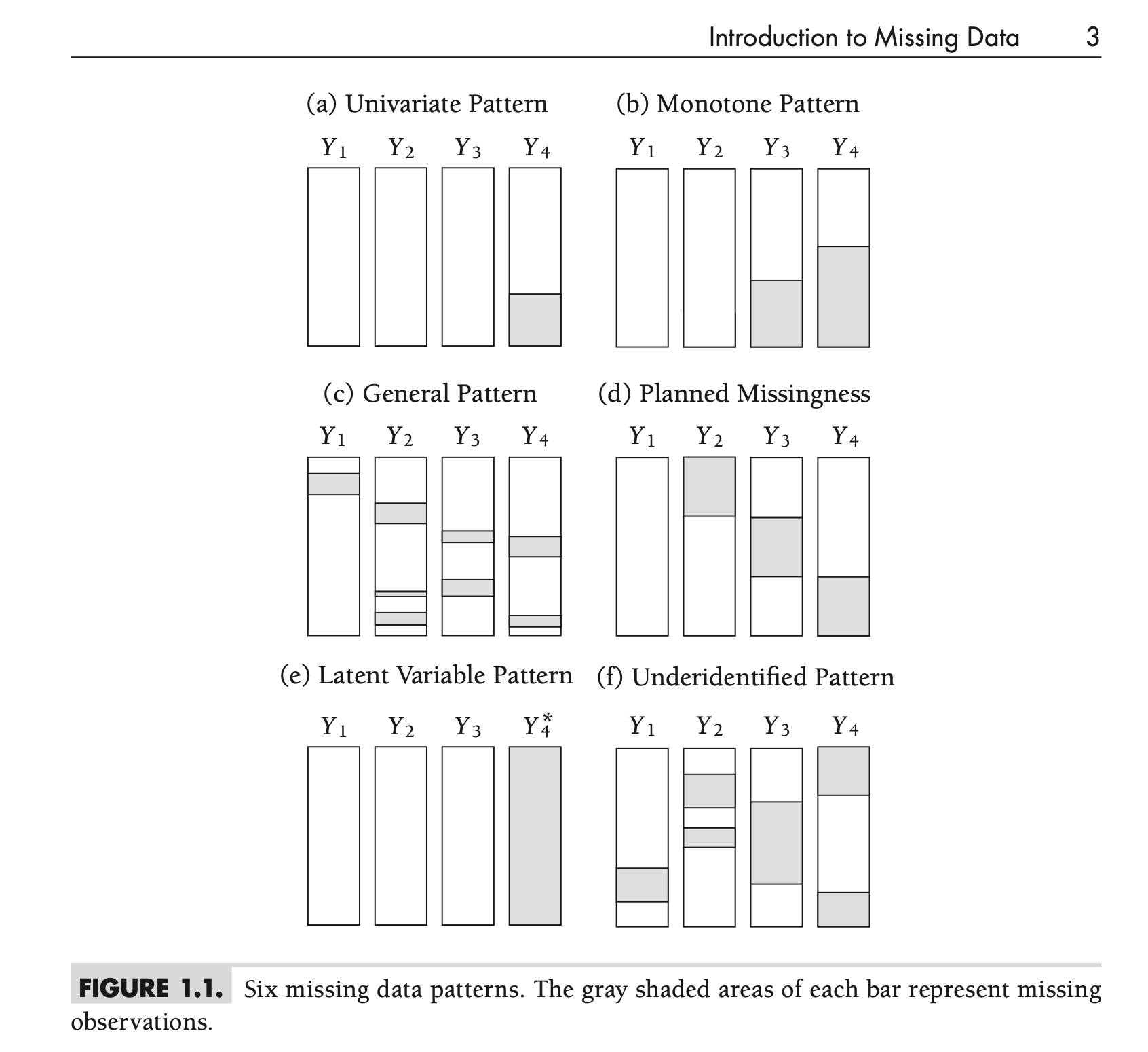
Univariate Pattern

• Missing values restricted to one variable
• Example: Missing outcomes for some participants

Monotone Pattern

• Missing data accumulates predictably
• Example: Dropout in longitudinal studies
• Can be treated without complicated iterative estimation algorithms

General Pattern

• Missing data scattered randomly across the dataset
• The three contemporary methods (maximum likelihood, Bayesian estimation, and multiple imputation) work well with this configuration
• Generally no reason to choose an analytic method based on the missing data pattern alone

Planned Missingness

• Variables are intentionally missing for a large proportion of respondents
• Can reduce respondent burden and research costs
• Often with minimal impact on statistical power

Latent Variable Pattern

• Latent variables are essentially missing data
  • Presents challenges in secondary analyses
• Example: Iowa wishes to understand how well an incoming student’s ACT score predicts first year GPA
  • ACT Score: An estimate–not an observation
    • Can think of scores as single imputation

Underidentified Pattern

• Insufficient overlap of data for estimation
• Example: Sparse cell counts for categorical variables

Missing Data Mechanisms

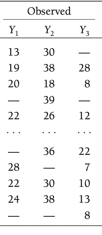
Hypothetical Data Partitioning: Observed Data

• Before getting to the types of missing data mechanisms, we must first define some notation
• Our observed data matrix will be defined as \(\mathbf{Y}_{(\text{obs})}\)
• Here, \(\mathbf{Y}_{(\text{obs})} = \left[Y_1, Y_2, Y_3 \right]\)

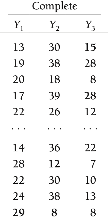
Hypothetical Data Partitioning: Complete Data

• Imagine if you could somehow see what the values of the missing data were – the complete data
• Our hypothetical data matrix will be defined as \(\mathbf{Y}_{(\text{com})}\) (sometimes denoted \(\mathbf{Y}_{(1)}\))
• Note: This is not possible through any method and is only a hypothetical example to help define missing data mechanisms

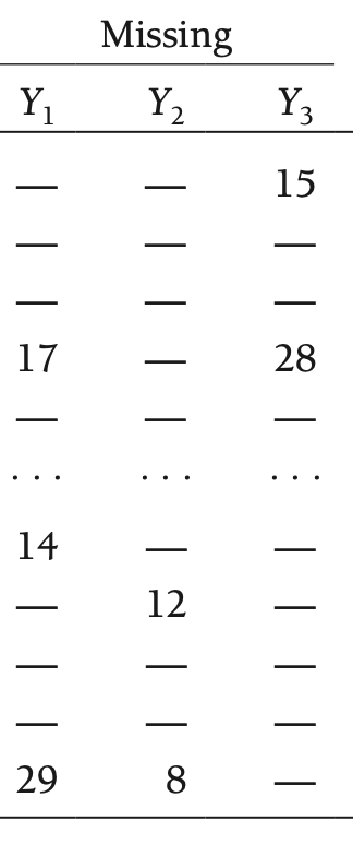
Hypothetical Data Partitioning: Missing Data

• Now, take the values that were missing and only create a matrix of those terms
• Our hypothetical data matrix will be defined as \(\mathbf{Y}_{(\text{mis})}\) (sometimes denoted \(\mathbf{Y}_{(0)}\))
• Note: Again, this is not possible through any method and is only a hypothetical example to help define missing data mechanisms

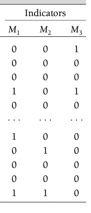
Rubin’s Framework

• Models that explain whether a participant has missing values
• How those tendencies relate to the realized data in \(\mathbf{Y}_{(\text{obs})}\) or \(\mathbf{Y}_{(\text{mis})}\)
• Here, \(\mathbf{M} = \left[M_1, M_2, M_3 \right]\)

Example Data

• To demonstrate some of the ideas of types of missing data, let’s consider a situation where you have collected two variables:
  • IQ scores
  • Job performance
• Imagine you are an employer looking to hire employees for a job where IQ is important

    IQ perfC
1   78     9
2   84    13
3   84    10
4   85     8
5   87     7
6   91     7
7   92     9
8   94     9
9   94    11
10  96     7
11  99     7
12 105    10
13 105    11
14 106    15
15 108    10
16 112    10
17 113    12
18 115    14
19 118    16
20 134    12

Missing Data Mechanisms

Missing Data Mechanisms

A very rough typology of missing data puts missing observations into three categories:

• Missing Completely At Random (MCAR)
• Missing At Random (MAR)
• Missing Not At Random (MNAR)

Missing Completely At Random (MCAR)

• Missing data are MCAR if the events that lead to missingness are independent of:
  • The observed variables
  • -and-
  • The unobserved parameters of interest
• Examples:
  • Planned missingness in survey research
    • Some large-scale tests are sampled using booklets
    • Students receive only a few of the total number of items
    • The items not received are treated as missing – but that is completely a function of sampling and no other mechanism

A Formal MCAR Definition

Formally, we note that data are MCAR if the probability of the data being missing is independent of the observed data \(\mathbf{Y}_{(obs)}\) and the missing data \(\mathbf{Y}_{(mis)}\):

\[Pr \left(\mathbf{M} = 1 \mid \mathbf{Y}_{(obs)}, \mathbf{Y}_{(mis)}, \boldsymbol{\phi} \right) = Pr \left(\mathbf{M} = 1 \mid \boldsymbol{\phi} \right)\]

• Here, \(\boldsymbol{\phi}\) are model parameters that define the overall probabilities of missing data
• Like saying a missing observation is due to pure randomness (such as missing if a coin flipped falls on heads)

Implications of MCAR

• Because the mechanism of missing is not due to anything other than chance, inclusion of MCAR in data will not bias your results
  • Can use methods based on listwise deletion, multiple imputation, or maximum likelihood
• Your effective sample size is lowered, though
  • Less power, less efficiency

MCAR Data

Missing data are dispersed randomly throughout data

    IQ perfMCAR
1   78       NA
2   84       13
3   84       NA
4   85        8
5   87        7
6   91        7
7   92        9
8   94        9
9   94       11
10  96       NA
11  99        7
12 105       10
13 105       11
14 106       15
15 108       10
16 112       NA
17 113       12
18 115       14
19 118       16
20 134       NA

MCAR vs. Complete Data Comparison

Complete Data

lavaan 0.6-19 ended normally after 20 iterations

  Estimator                                         ML
  Optimization method                           NLMINB
  Number of model parameters                         5

  Number of observations                            20

Model Test User Model:
                                                      
  Test statistic                                 0.000
  Degrees of freedom                                 0

Parameter Estimates:

  Standard errors                             Standard
  Information                                 Expected
  Information saturated (h1) model          Structured

Covariances:
                   Estimate  Std.Err  z-value  P(>|z|)   Std.lv  Std.all
  IQ ~~                                                                 
    perfC            19.500    9.151    2.131    0.033   19.500    0.542

Intercepts:
                   Estimate  Std.Err  z-value  P(>|z|)   Std.lv  Std.all
    IQ              100.000    3.079   32.478    0.000  100.000    7.262
    perfC            10.350    0.584   17.714    0.000   10.350    3.961

Variances:
                   Estimate  Std.Err  z-value  P(>|z|)   Std.lv  Std.all
    IQ              189.600   59.957    3.162    0.002  189.600    1.000
    perfC             6.828    2.159    3.162    0.002    6.828    1.000

MAR Data

lavaan 0.6-19 ended normally after 20 iterations

  Estimator                                         ML
  Optimization method                           NLMINB
  Number of model parameters                         5

  Number of observations                            15

Model Test User Model:
                                                      
  Test statistic                                 0.000
  Degrees of freedom                                 0

Parameter Estimates:

  Standard errors                             Standard
  Information                                 Expected
  Information saturated (h1) model          Structured

Covariances:
                   Estimate  Std.Err  z-value  P(>|z|)   Std.lv  Std.all
  IQ ~~                                                                 
    perfMCAR         19.360    9.299    2.082    0.037   19.360    0.638

Intercepts:
                   Estimate  Std.Err  z-value  P(>|z|)   Std.lv  Std.all
    IQ               99.733    2.777   35.916    0.000   99.733    9.274
    perfMCAR         10.600    0.729   14.539    0.000   10.600    3.754

Variances:
                   Estimate  Std.Err  z-value  P(>|z|)   Std.lv  Std.all
    IQ              115.662   42.234    2.739    0.006  115.662    1.000
    perfMCAR          7.973    2.911    2.739    0.006    7.973    1.000

Missing at Random Definition

Formally, we note that data are MAR if the probability of the data being missing is related to the observed data \(\mathbf{Y}_{(obs)}\) but not the missing data \(\mathbf{Y}_{(mis)}\):

\[Pr \left(\mathbf{M} = 1 \mid \mathbf{Y}_{(obs)}, \mathbf{Y}_{(mis)}, \boldsymbol{\phi} \right) = Pr \left(\mathbf{M} = 1 \mid \mathbf{Y}_{(obs)}, \boldsymbol{\phi} \right)\]

• Again, \(\boldsymbol{\phi}\) are model parameters that define the overall probabilities of missing data
• Like saying a missing observation is due to pure randomness (such as missing if a coin flipped falls on heads)

MAR Data

Missing data are related to other data:

• Any IQ less than 90 did not have a performance variable
  • Could be that anyone with an IQ of 90 or less was not hired
  • Not hired means not having job performance data

    IQ perfMAR
1   78      NA
2   84      NA
3   84      NA
4   85      NA
5   87      NA
6   91       7
7   92       9
8   94       9
9   94      11
10  96       7
11  99       7
12 105      10
13 105      11
14 106      15
15 108      10
16 112      10
17 113      12
18 115      14
19 118      16
20 134      12

Implications of MAR

• If data are missing at random, biased results could occur
• Inferences based on listwise deletion will be biased and inefficient
  • Fewer data points = more error in analysis
• Inferences based on maximum likelihood will be unbiased but inefficient
• The first eight chapters of the book focus on methods for MAR data

MAR vs. Complete Data Comparison

Complete Data

lavaan 0.6-19 ended normally after 20 iterations

  Estimator                                         ML
  Optimization method                           NLMINB
  Number of model parameters                         5

  Number of observations                            20

Model Test User Model:
                                                      
  Test statistic                                 0.000
  Degrees of freedom                                 0

Parameter Estimates:

  Standard errors                             Standard
  Information                                 Expected
  Information saturated (h1) model          Structured

Covariances:
                   Estimate  Std.Err  z-value  P(>|z|)   Std.lv  Std.all
  IQ ~~                                                                 
    perfC            19.500    9.151    2.131    0.033   19.500    0.542

Intercepts:
                   Estimate  Std.Err  z-value  P(>|z|)   Std.lv  Std.all
    IQ              100.000    3.079   32.478    0.000  100.000    7.262
    perfC            10.350    0.584   17.714    0.000   10.350    3.961

Variances:
                   Estimate  Std.Err  z-value  P(>|z|)   Std.lv  Std.all
    IQ              189.600   59.957    3.162    0.002  189.600    1.000
    perfC             6.828    2.159    3.162    0.002    6.828    1.000

MAR Data

lavaan 0.6-19 ended normally after 21 iterations

  Estimator                                         ML
  Optimization method                           NLMINB
  Number of model parameters                         5

  Number of observations                            15

Model Test User Model:
                                                      
  Test statistic                                 0.000
  Degrees of freedom                                 0

Parameter Estimates:

  Standard errors                             Standard
  Information                                 Expected
  Information saturated (h1) model          Structured

Covariances:
                   Estimate  Std.Err  z-value  P(>|z|)   Std.lv  Std.all
  IQ ~~                                                                 
    perfMAR          19.489    9.413    2.070    0.038   19.489    0.633

Intercepts:
                   Estimate  Std.Err  z-value  P(>|z|)   Std.lv  Std.all
    IQ              105.467    2.947   35.791    0.000  105.467    9.241
    perfMAR          10.667    0.697   15.302    0.000   10.667    3.951

Variances:
                   Estimate  Std.Err  z-value  P(>|z|)   Std.lv  Std.all
    IQ              130.249   47.560    2.739    0.006  130.249    1.000
    perfMAR           7.289    2.662    2.739    0.006    7.289    1.000

Missing Not At Random (MNAR) Definition

Formally, we note that data are MNAR if the probability of the data being missing is related to the observed data \(\mathbf{Y}_{(obs)}\) and the missing data \(\mathbf{Y}_{(mis)}\):

\[Pr \left(\mathbf{M} = 1 \mid \mathbf{Y}_{(obs)}, \mathbf{Y}_{(mis)}, \boldsymbol{\phi} \right)\]

• Again, \(\boldsymbol{\phi}\) are model parameters that define the overall probabilities of missing data

Often called non-ignorable missingness

• Inferences based on listwise deletion or maximum likelihood will be biased and inefficient
• Need to provide statistical model for missing data simultaneously with estimation of original model

Surviving Missing data: A Brief Guide

Using Statistical Methods with Missing Data

• Missing data can alter your analysis results dramatically depending upon:
  • 1. The type of missing data
  • 2. The type of analysis algorithm
• The choice of an algorithm and missing data method is important in avoiding issues due to missing data

The Worst Case Scenario: MNAR

• The worst case scenario is when data are MNAR: missing not at random
  • Non-ignorable missing
• You cannot easily get out of this mess
  • Instead you have to be clairvoyant
• Analyses algorithms must incorporate models for missing data
  • And these models must also be right

The Reality

• In most empirical studies, MNAR as a condition is an afterthought
• It is impossible to know definitively if data truly are MNAR
  • So data are treated as MAR or MCAR
• Hypothesis tests do exist for MCAR (i.e., Little’s test)
  • But, often this test is rejected

The Best Case Scenario: MCAR

• Under MCAR, pretty much anything you do with your data will give you the “right” (unbiased) estimates of your model parameters
• MCAR is very unlikely to occur
  • In practice, MCAR is treated as equally unlikely as MNAR

The Middle Ground: MAR

• MAR is the common compromise used in most empirical research
  • Under MAR, maximum likelihood algorithms are unbiased
• Maximum likelihood is for many methods:
  • Linear mixed models i
  • Models with “latent” random effects (CFA/SEM models)

Outdated Methods for Handling Missing Data

Bad Ways to Handle Missing Data

• Dealing with missing data is important, as the mechanisms you choose can dramatically alter your results
• This point was not fully realized when the first methods for missing data were created
  • Each of the methods described in this section should never be used
  • Given to show perspective – and to allow you to understand what happens if you were to choose each

Deletion Methods

• Deletion methods are just that: methods that handle missing data by deleting observations
  • Listwise deletion: delete the entire observation if any values are missing
  • Pairwise deletion: delete a pair of observations if either of the values are missing
• Assumptions: Data are MCAR
• Limitations:
  • Reduction in statistical power if MCAR
  • Biased estimates if MAR or MNAR

Listwise Deletion

• Listwise deletion discards all of the data from an observation if one or more variables are missing
• Most frequently used in statistical software packages that are not optimizing a likelihood function (need ML)
• In linear models:
  • R lm() list-wise deletes cases where DVs are missing

Listwise Deletion Example: MCAR

Parameter Estimates:

  Standard errors                             Standard
  Information                                 Expected
  Information saturated (h1) model          Structured

Regressions:
                   Estimate  Std.Err  z-value  P(>|z|)
  perfC ~                                             
    IQ                0.103    0.036    2.884    0.004

Intercepts:
                   Estimate  Std.Err  z-value  P(>|z|)
   .perfC             0.065    3.600    0.018    0.986

Variances:
                   Estimate  Std.Err  z-value  P(>|z|)
   .perfC             4.822    1.525    3.162    0.002

Parameter Estimates:

  Standard errors                             Standard
  Information                                 Expected
  Information saturated (h1) model          Structured

Regressions:
                   Estimate  Std.Err  z-value  P(>|z|)
  perfMCAR ~                                          
    IQ                0.167    0.052    3.205    0.001

Intercepts:
                   Estimate  Std.Err  z-value  P(>|z|)
   .perfMCAR         -6.094    5.239   -1.163    0.245

Variances:
                   Estimate  Std.Err  z-value  P(>|z|)
   .perfMCAR          4.733    1.728    2.739    0.006

Listwise Deletion Example: MAR

Parameter Estimates:

  Standard errors                             Standard
  Information                                 Expected
  Information saturated (h1) model          Structured

Regressions:
                   Estimate  Std.Err  z-value  P(>|z|)
  perfC ~                                             
    IQ                0.103    0.036    2.884    0.004

Intercepts:
                   Estimate  Std.Err  z-value  P(>|z|)
   .perfC             0.065    3.600    0.018    0.986

Variances:
                   Estimate  Std.Err  z-value  P(>|z|)
   .perfC             4.822    1.525    3.162    0.002

Parameter Estimates:

  Standard errors                             Standard
  Information                                 Expected
  Information saturated (h1) model          Structured

Regressions:
                   Estimate  Std.Err  z-value  P(>|z|)
  perfMAR ~                                           
    IQ                0.150    0.047    3.163    0.002

Intercepts:
                   Estimate  Std.Err  z-value  P(>|z|)
   .perfMAR          -5.114    5.019   -1.019    0.308

Variances:
                   Estimate  Std.Err  z-value  P(>|z|)
   .perfMAR           4.373    1.597    2.739    0.006

Pairwise Deletion

• Pairwise deletion discards a pair of observations if either one is missing
  • Different from listwise: uses more data (rest of data not thrown out)
• Assumes: MCAR
• Limitations:
  • Reduction in statistical power if MCAR
  • Biased estimates if MAR or MNAR
• Can be an issue when forming covariance/correlation matrices
  • May make them non-invertible, problem if used as input into statistical procedures

Pairwise Deletion Example

cor(jobPerf, use="pairwise.complete.obs")

                IQ     perfC  perfMCAR   perfMAR
IQ       1.0000000 0.5419817 0.6375139 0.6325129
perfC    0.5419817 1.0000000 1.0000000 1.0000000
perfMCAR 0.6375139 1.0000000 1.0000000 1.0000000
perfMAR  0.6325129 1.0000000 1.0000000 1.0000000

Single Imputation Methods

• Single imputation methods replace missing data with some type of value
  • Single: one value used
  • Imputation: replace missing data with value
• Upside: can use entire data set if missing values are replaced
• Downside: biased parameter estimates and standard errors (even if missing is MCAR)
  • Type-I error issues
• Still: never use these techniques

Unconditional Mean Imputation

• Unconditional mean imputation replaces the missing values of a variable with its estimated mean
  • Unconditional = mean value without any input from other variables

Unconditional Mean Imputation: MCAR Data vs Complete Data

Complete

Call:
lm(formula = perfC ~ IQ, data = jobPerf)

Residuals:
    Min      1Q  Median      3Q     Max 
-3.2472 -1.6498 -0.6301  1.2742  4.2956 

Coefficients:
            Estimate Std. Error t value Pr(>|t|)  
(Intercept)  0.06519    3.79433   0.017   0.9865  
IQ           0.10285    0.03759   2.736   0.0136 *
---
Signif. codes:  0 '***' 0.001 '**' 0.01 '*' 0.05 '.' 0.1 ' ' 1

Residual standard error: 2.315 on 18 degrees of freedom
Multiple R-squared:  0.2937,    Adjusted R-squared:  0.2545 
F-statistic: 7.487 on 1 and 18 DF,  p-value: 0.01357

MCAR

Call:
lm(formula = perfMCAR_meanImpute ~ IQ, data = jobPerf)

Residuals:
    Min      1Q  Median      3Q     Max 
-3.5234 -1.2723 -0.4509  1.3402  4.0215 

Coefficients:
            Estimate Std. Error t value Pr(>|t|)  
(Intercept)  2.94177    3.81241   0.772   0.4503  
IQ           0.07658    0.03777   2.028   0.0577 .
---
Signif. codes:  0 '***' 0.001 '**' 0.01 '*' 0.05 '.' 0.1 ' ' 1

Residual standard error: 2.326 on 18 degrees of freedom
Multiple R-squared:  0.1859,    Adjusted R-squared:  0.1407 
F-statistic: 4.112 on 1 and 18 DF,  p-value: 0.05766

Unconditional Mean Imputation: MAR Data vs Complete Data

Complete

Call:
lm(formula = IQ ~ perfC, data = jobPerf)

Residuals:
    Min      1Q  Median      3Q     Max 
-23.569  -7.425   1.216   6.572  29.287 

Coefficients:
            Estimate Std. Error t value Pr(>|t|)    
(Intercept)   70.439     11.143   6.322 5.87e-06 ***
perfC          2.856      1.044   2.736   0.0136 *  
---
Signif. codes:  0 '***' 0.001 '**' 0.01 '*' 0.05 '.' 0.1 ' ' 1

Residual standard error: 12.2 on 18 degrees of freedom
Multiple R-squared:  0.2937,    Adjusted R-squared:  0.2545 
F-statistic: 7.487 on 1 and 18 DF,  p-value: 0.01357

MAR

Call:
lm(formula = IQ ~ perfMAR_meanImpute, data = jobPerf)

Residuals:
    Min      1Q  Median      3Q     Max 
-22.000  -8.418   2.272   7.288  30.435 

Coefficients:
                   Estimate Std. Error t value Pr(>|t|)    
(Intercept)          71.480     13.506   5.293 4.95e-05 ***
perfMAR_meanImpute    2.674      1.237   2.162   0.0443 *  
---
Signif. codes:  0 '***' 0.001 '**' 0.01 '*' 0.05 '.' 0.1 ' ' 1

Residual standard error: 12.93 on 18 degrees of freedom
Multiple R-squared:  0.2061,    Adjusted R-squared:  0.162 
F-statistic: 4.674 on 1 and 18 DF,  p-value: 0.04434

Conditional Mean Imputation (Regression)

• Conditional mean imputation uses regression analyses to impute missing values
  • The missing values are imputed using the predicted values in each regression (conditional means)
• For our data we would form regressions for each outcome using the other variables
  • PERF = β01 + β11*IQ
• More accurate than unconditional mean imputation
  • But still provides biased parameters and SEs

Stochastic Conditional Mean Imputation

• Stochastic conditional mean imputation adds a random component to the imputation
  • Representing the error term in each regression equation
  • Assumes MAR rather than MCAR
• Better than any other of these methods (and the basis for multiple imputation)

Imputation by Proximity: Hot Deck Matching

• Hot deck matching uses real data – from other observations as its basis for imputing
• Observations are “matched” using similar scores on variables in the data set
  • Imputed values come directly from matched observations
• Upside: Helps to preserve univariate distributions; gives data in an appropriate range
• Downside: biased estimates (especially of regression coefficients), too-small standard errors

Scale Imputation by Averaging

• In psychometric tests, a common method of imputation has been to use a scale average rather than total score
  • Can re-scale to total score by taking # items * average score
• Problem: treating missing items this way is like using person mean
  • Reduces standard errors
  • Makes calculation of reliability biased

Longitudinal Imputation: Last Observation Carried Forward

• A commonly used imputation method in longitudinal data has been to treat observations that dropped out by carrying forward thelast observation
  • More common in medical studies and clinical trials
• Assumes scores do not change after dropout – bad idea
  • Thought to be conservative
• Can exaggerate group differences
  • Limits standard errors that help detect group differences

Why Single Imputation Is Bad Science

• Overall, the methods described in this section are not useful for handling missing data
• If you use them you will likely get a statistical answer that is an artifact
  • Actual estimates you interpret (parameter estimates) will be biased (in either direction)
  • Standard errors will be too small
    • Leads to Type-I Errors
• Putting this together: you will likely end up making conclusions about your data that are wrong

Auxiliary Variables and Semi-Partial Correlation

Auxiliary Variables and Semi-Partial Correlation

The use of auxiliary variables can help mitigate bias and improve statistical power when missing data are present

• An auxiliary variable is an extraneous variable that correlates with missingness or the outcome but is not part of the main analysis

A key aspect of auxiliary variable selection is understanding their semi-partial correlation with the outcome

• Semi-partial correlation quantifies the unique contribution of a predictor to the outcome, after removing its shared variance with other predictors
• This makes Semi-partial correlations useful for identifying the most informative auxiliary variables

What is a Semi-Partial Correlation?

• Semi-partial correlation (also known as part correlation) measures the unique association between a predictor and the outcome while controlling for other variables in the model
• Unlike partial correlation, which removes shared variance from both variables, semi-partial correlation removes shared variance only from the predictor variable, leaving the outcome variable unchanged

What is a Semi-Partial Correlation?

Mathematically, the semi-partial correlation of a predictor \(( X_1 )\) with an outcome \((Y)\), controlling for another predictor \(X_2\), is given by:

\[ r_{Y(X_1.X_2)} = \frac{r_{YX_1} - r_{YX_2}r_{X_1X_2}}{\sqrt{1 - r_{X_1X_2}^2}} \]

where: - \(r_{YX_1}\)is the correlation between \(Y\) and \(X_1\), - \(r_{YX_2}\) is the correlation between \(Y\) and \(X_2\), - \(r_{X_1X_2}\) is the correlation between \(X_1\) and \(X_2\).

Why is Semi-Partial Correlation Important?

Semi-partial correlation is widely used in statistics for several reasons:

1. Understanding Unique Contributions – It helps to determine how much unique variance a predictor explains in the outcome, which is useful in multiple regression and hierarchical modeling
2. Feature Selection – In machine learning and predictive modeling, semi-partial correlation can help identify the most important predictors
3. Model Interpretation – Researchers can use it to assess the relative importance of predictors in explaining variance in an outcome
4. Comparing Predictors – It allows us to compare multiple predictors to see which has the most unique explanatory power

Because semi-partial correlation removes shared variance only from the predictor, it reflects the real-world scenario where some predictors contribute uniquely to an outcome while sharing variance with others.

Semi-Partial Correlation in the Context of Missing Data

• Semi-partial correlations help identify which auxiliary variables provide unique information about missingness or the outcome
  • This ensures that missing data handling methods, such as multiple imputation or maximum likelihood estimation, make the most use of available information

Example in R

Simulated Data

Let’s create a dataset where we examine semi-partial correlations:

set.seed(42)
n = 100
y = rnorm(n, mean=50, sd=10)   # Outcome variable
x1 = rnorm(n, mean=10, sd=5)    # Predictor 1
x2 = rnorm(n, mean=20, sd=5)    # Predictor 2
aux = .05*y + 0.5*x1 + 0.3*x2 + rnorm(n, mean=0, sd=2)  # Auxiliary variable

data = data.frame(y, x1, x2, aux)

Computing Semi-Partial Correlation using lm() residuals

# Step 1: Regress the auxiliary variable on other predictors and obtain residuals
aux_resid = resid(lm(aux ~ x1 + x2, data=data))

# Step 2: Compute the correlation between residuals and the outcome
spr_lm = cor(aux_resid, data$y)
print(spr_lm)

[1] 0.3371851

Computing Semi-Partial Correlation using the ppcor package

# Compute semi-partial correlation using spcorr package
spr_spcorr = spcor(data)
print(spr_spcorr)

$estimate
             y         x1         x2       aux
y    1.0000000 -0.2359666 -0.3182904 0.3371851
x1  -0.1543577  1.0000000 -0.3222919 0.7896905
x2  -0.2605867 -0.4033669  1.0000000 0.6280408
aux  0.1904317  0.6817890  0.4332414 1.0000000

$p.value
              y           x1           x2          aux
y   0.000000000 1.932959e-02 1.403247e-03 6.859535e-04
x1  0.129123301 0.000000e+00 1.210448e-03 4.366625e-22
x2  0.009555429 3.816958e-05 0.000000e+00 4.454870e-12
aux 0.060351647 1.092502e-14 8.354724e-06 0.000000e+00

$statistic
            y        x1        x2       aux
y    0.000000 -2.379176 -3.289682  3.509232
x1  -1.530736  0.000000 -3.335800 12.611715
x2  -2.644587 -4.319133  0.000000  7.907571
aux  1.900622  9.131503  4.709848  0.000000

$n
[1] 100

$gp
[1] 2

$method
[1] "pearson"

Comparison of Results

Both methods should yield similar results, but spcor provides a more automated way to compute semi-partial correlations, making it easier to handle multiple predictors at once.

• But, ‘spcor’ doesn’t have the ability to specify certain combinations of variables

Interpretation:

• If the semi-partial correlation is strong (e.g., above 0.30 in absolute value), the auxiliary variable is likely to contain unique information about the outcome and should be included in the missing data handling process

Wrapping Up

Lecture Summary

• Missing data are common in statistical analyses
• They are frequently neglected
  • MNAR: hard to model missing data and observed data simultaneously
  • MCAR: doesn’t often happen
  • MAR: most missing imputation assumes MVN
• More often than not, ML is the best choice
  • Software is getting better at handling missing data
  • We will discuss how ML works next week