Model Fit
Today’s Lecture
- The logic of model fit
- Absolute vs. relative fit
- Why model fit is important
- (Dis)confirming the hypothesized Q-matrix
- Implications for validity
- Fit to target distribution
- Model fit in MML CFA models (and Limited Information Estimation in MIRT)
- Derivation of model-implied covariance matrix
- Model fit statistics
- Model fit in MML IRT models
- M2 statistics and derivatives
- Bayesian Model Fit (and model fit for cases where established methods are not available)
- Posterior predictive model checking
- Target statistics
The Logic of Model Fit
- Model fit is the process of determining whether the model is consistent with the data or whether one model is preferable to another
- Types of Model Fit
- Absolute fit: How well does the model fit the data?
- Relative fit: Which of a set of models fits the data better?
- In relative fit, all models being compared must have good absolute fit to the data
Why Model Fit is Important
If a model does not fit the data:
- Parameter estimates may be biased
- Standard errors of estimates may be biased (posterior SDs in Bayesian models)
- Inferences made from the model may be wrong
- Scores based on the model may be wrong (and have incorrect conditional standard errors)
Examining model fit is the first step after estimation in psychometric models
That said, not all “good-fitting” models are useful…
- …model fit just allows you to talk about your model…there may be nothing of significance (statistically or practically) in your results, though
Model Fit and the Q-Matrix
- The process of model fit can be placed into a hypothesis testing statistical framework
- The null hypothesis is that the model is correct (i.e., the Q-matrix is correct)
- The alternative hypothesis is that the model is incorrect
- Specifically, that a saturated model fits better
Model Fit: First Steps in a Validity Argument
- If a model does not fit the data, the scores and their standard errors are likely to have some degree of bias
- Therefore, validity of scores cannot be established if the model does not fit the data
- Model fit is the first step in a validity argument
- I like to call model fit consequential validity
Model Fit and a Target Distribution
- The key to understanding model fit is to understand the target distribution
- The target distribution is the distribution of the data that the model is trying to reproduce
- In MML models, the target distribution is the distribution of the data that would be obtained if the model were correct
- In Bayesian models, the target distribution is the posterior predictive distribution
- Not all models have easily identifiable target distributions (e.g., models where observed variables have differing distributions)
- In these cases, model fit is more difficult to assess
From CFA to Target Distribution
We will begin by examining our CFA model and deriving the model-implied covariance matrix
\[ Y_{pi} = \mu_i + \sum_{d=1}^D q_{id} \lambda_{id} \theta_{pd} + e_{pi}\]
Where:
- \(Y_{pi}\) is the response for person \(p\) on item \(i\)
- \(e_{pi} \sim N\left(0, \psi^2_i \right)\) is the error term for person \(p\) on item \(i\)
- \(\psi^2_i\) is the unique variance of the error term
- \(\mu_i\) is the item intercept
- \(\lambda_{id}\) is the item loading/slope for item \(i\) and latent variable \(d\)
- \(\theta_{pd}\) is the latent variable score for person \(p\) and latent variable \(d\)
- \(D\) is the number of latent variables
- \(q_{id}\) is the Q-matrix entry for item \(i\) and latent variable \(d\)
From One Item to Many
A model is specified a collection of items, making it a multivariate model:
\[ \begin{array}{cc} Y_{p1} = \mu_1 + \sum_{d=1}^D q_{1d} \lambda_{1d} \theta_{pd} + e_{p, 1}; & e_{p,1} \sim N\left(0, \psi_1^2 \right) \\ Y_{p2} = \mu_2 + \sum_{d=1}^D q_{2d} \lambda_{2d} \theta_{pd} + e_{p, 2}; & e_{p,2} \sim N\left(0, \psi_2^2 \right) \\ \vdots \\ Y_{pI} = \mu_I + \sum_{d=1}^D q_{Id} \lambda_{Id} \theta_{pd} + e_{p, I}; & e_{p,I} \sim N\left(0, \psi_I^2 \right) \\ \end{array} \]
From Scalar Equations to Matrix Equations
We can write the model in matrix form:
\[ \begin{array}{cc} \boldsymbol{Y}_p = \boldsymbol{\mu} + \boldsymbol{\Lambda}_\boldsymbol{Q} \boldsymbol{\theta}_p + \boldsymbol{e}_p; & \boldsymbol{e}_p \sim N\left(\boldsymbol{0}, \boldsymbol{\Psi} \right) \\ \end{array} \]
Where:
- \(I\) is the number of items, \(D\) is the number of latent variables
- \(\boldsymbol{Y}_p\) is an \(I \times 1\) vector of responses for person \(p\)
- \(\boldsymbol{\mu}\) is an \(I \times 1\) vector of item intercepts
- \(\boldsymbol{\Lambda}_\boldsymbol{Q}\) is the \(D \times I\) matrix of item loadings where \(\lambda_{id} = 0\) if \(q_{id} = 0\)
- \(\boldsymbol{\theta}_p\) is the \(D \times 1\) vector of latent variable scores for person \(p\), with \(\boldsymbol{\theta}_p \sim N\left(\boldsymbol{\mu}_{\theta}, \boldsymbol{\Phi} \right)\)
- \(\boldsymbol{\mu}_{\theta}\) is the vector of latent variable means (frequently set to zero for identification)
- \(\boldsymbol{\Phi}\) is the \(D \times D\) covariance matrix of the latent variables
- \(\boldsymbol{e}_p\) is the \(I \times 1\) vector of error terms for person \(p\)
- \(\boldsymbol{\Psi}\) is the \(I \times I\) diagonal matrix of unique variances
From Matrix Equations to the Model-Implied Distribution
Assuming that the latent variable scores are normally distributed, the model-implied conditional distribution is:
\[ \begin{array}{cc} f \left( \boldsymbol{Y}_p \mid \boldsymbol{\theta}_p \right) \sim N\left(\boldsymbol{\mu} + \boldsymbol{\Lambda}_\boldsymbol{Q} \boldsymbol{\theta}_p, \boldsymbol{\Psi} \right) \\ \end{array} \]
- But, this is only the first step as need \(f \left( \boldsymbol{Y}_p\right)\) (the marginal distribution of the data)
A Quick Note About Types of Distributions
- For two random variables \(x\) and \(z\), a conditional distribution is written as: \(f\left(x \mid z \right)\)
- The conditional distribution is also equal to the joint distribution divided by the marginal distribution of the conditioning random variable
\[ f\left(x \mid z \right) = \frac{f\left(x, z \right)}{f\left(z \right)} \]
- Therefore, the joint distribution can be found by the product of the conditional and marginal distributions:
\[ f\left(x, z \right) = f\left(x \mid z \right) f\left(z \right) \]
- We can use this result in our model-implied distribution to find the marginal distribution of the data
\[f \left( \boldsymbol{Y}_p \mid \boldsymbol{\theta}_p \right) f \left( \boldsymbol{\theta}_p \right) = f \left( \boldsymbol{Y}_p , \boldsymbol{\theta}_p \right)\]
The Marginal Distribution of the Data
- The marginal distribution of the data is found by integrating over the latent variable scores
\[ \begin{array}{cc} f \left( \boldsymbol{Y}_p \right) = \int_{\boldsymbol{\theta}_p} f \left( \boldsymbol{Y}_p , \boldsymbol{\theta}_p \right) d \boldsymbol{\theta}_p \\ \end{array} \]
- While this seems difficult due to the integral, the multivariate normal distribution has a nice property that makes this integral solvable in closed form
Properties of the Multivariate Normal Distribution
- If \(\boldsymbol{X}\) is distributed multivariate normally, conditional and marginal distributions of \(\boldsymbol{X}\) are multivariate normal
- Why this matters: we can show that \(f \left( \boldsymbol{Y}_p \right)\) is MVN:
\[f \left( \boldsymbol{Y}_p \right) \sim N \left(? , ? \right)\]
- We can determine the paramater matrices using the algebra of expected values
Algebra of Expectations
The mean of our model-implied distribution is:
\[ E \left[ \boldsymbol{Y}_p \right] = E \left[ \boldsymbol{\mu} + \boldsymbol{\Lambda}_\boldsymbol{Q} \boldsymbol{\theta}_p + \boldsymbol{e}_p \right] = \boldsymbol{\mu} + \boldsymbol{\Lambda}_\boldsymbol{Q} E \left[ \boldsymbol{\theta}_p \right] + E \left[ \boldsymbol{e}_p \right] = \boldsymbol{\mu} + \boldsymbol{\Lambda}_\boldsymbol{Q} \boldsymbol{\mu}_\theta \]
So, we know:
\[f \left( \boldsymbol{Y}_p \right) \sim N \left(\boldsymbol{\mu} + \boldsymbol{\Lambda}_\boldsymbol{Q} \boldsymbol{\mu}_\theta, ? \right)\]
Model-Implied Covariance Matrix
The covariance matrix of our model-implied distribution is:
\[ Var \left[ \boldsymbol{Y}_p \right] = Var \left[ \boldsymbol{\mu} + \boldsymbol{\Lambda}_\boldsymbol{Q} \boldsymbol{\theta}_p \right] = Var \left[ \boldsymbol{\Lambda}_\boldsymbol{Q} \boldsymbol{\theta}_p \right] + Var \left[ \boldsymbol{e}_p \right] = \boldsymbol{\Lambda}_\boldsymbol{Q} \boldsymbol{\Phi} \boldsymbol{\Lambda}_\boldsymbol{Q}^T + \boldsymbol{\Psi} \]
Model Implied Data Distribution
Therefore, the CFA model-implied distribution (the marginal distribution of the data) is:
\[f \left( \boldsymbol{Y}_p \right) \sim N \left(\boldsymbol{\mu} + \boldsymbol{\Lambda}_\boldsymbol{Q} \boldsymbol{\mu}_\theta, \boldsymbol{\Lambda}_\boldsymbol{Q} \boldsymbol{\Phi} \boldsymbol{\Lambda}_\boldsymbol{Q}^T + \boldsymbol{\Psi} \right)\]
Which, when \(\boldsymbol{\mu}_\theta = \boldsymbol{0}\) becomes:
\[f \left( \boldsymbol{Y}_p \right) \sim N \left(\boldsymbol{\mu} , \boldsymbol{\Lambda}_\boldsymbol{Q} \boldsymbol{\Phi} \boldsymbol{\Lambda}_\boldsymbol{Q}^T + \boldsymbol{\Psi} \right)\]
Target Distribution
Now that we know the model-implied distribution, we can determine the target distribution
- The target distribution is the distribution that would subsume our model
- In other words, a distribution within which all CFA-type models would be nested
- In the case where all items follow the CFA model, the target distribution is a saturated MVN distribution
\[f \left( \boldsymbol{Y}_p \right) \sim N \left(\boldsymbol{\mu}_{1} , \boldsymbol{\Sigma}_1 \right)\]
Where:
- \(\boldsymbol{\mu}_{1}\) is the \(I \times 1\) vector of item means (not CFA model means)
- \(\boldsymbol{\Sigma}_1\) is the \(I \times I\) covariance matrix of the items (not CFA model covariance matrix)
Examining the Target Distribution: The Mean
- As the target distribution is MVN with two parameter matrices, we can compare the two to our CFA model to better understand model fit
The target distribution mean, \(\boldsymbol{\mu}_{1}\) can be comarped to the CFA model mean, \(\boldsymbol{\mu} + \boldsymbol{\Lambda}_\boldsymbol{Q} \boldsymbol{\mu}_\theta\)
- When \(\boldsymbol{\mu}_\theta = \boldsymbol{0}\), the target distribution mean is equal to the CFA model mean
- Therefore, in most CFA applications, the mean fits perfectly as it is saturated
Examining the Target Distribution: The Covariance Matrix
The target distribution covariance matrix, \(\boldsymbol{\Sigma}_1\) can be comarped to the CFA model covariance matrix, \(\boldsymbol{\Lambda}_\boldsymbol{Q} \boldsymbol{\Phi} \boldsymbol{\Lambda}_\boldsymbol{Q}^T + \boldsymbol{\Psi}\)
More specifically, the variance of any given item, \(i\), from the target distribution is \(\sigma_{1i}^2\)
Our model-implied variance is \(\boldsymbol{\lambda}_{\boldsymbol{Q},i} \boldsymbol{\Phi} \boldsymbol{\lambda}_{\boldsymbol{Q},i}^T + \boldsymbol{\psi}_i\)
Here, if we allow all \(\boldsymbol{\psi}_i\) to be estimated (saturated), the diagnonal of the target distribution covariance matrix is equal to the diagnonal of the model-implied covariance matrix
Therefore, model fit is determined by the off-diagonal elements of the covariance matrix
Model Fit Methods
- Absolute model fit can be assessed
- Globally (across all of the data in the model), producing a single model fit statistic (one of many )
- Locally (for given elements of the covariance matrix), evaluating fit for a pair of items
- Methods for model fit vary by types of estimation
- Maximum Likelihood CFA:
- Many global statistics are available
- Local fit assessed by raw, standardized, and studentized residuals
- Maximum Likelihood CFA:
- In Bayesian CFA:
- Fewer global statistics are available
- Posterior predictive model checking used for almost everything
Global ML-Based Model Fit Statistics
- There are many model fit statistics that can be used to assess model fit
- The most common are:
- Chi-square test statistic (rarely used)
- Root mean square error of approximation (RMSEA; historically want to be < .05)
- Comparative fit index (CFI; historically want to be > .95)
- Tucker-Lewis index (TLI; historically want to be > .95)
- Standardized root mean square residual (SRMR; historically want to be < .08)
- SRMR uses the standardized residuals of the covariance matrix to assess model fit
Good reference for current thinking on each:
West, S. G., Wu, W., McNeish, D., & Savord, A. (2023). Model fit in structural equation modeling. In R. H. Hoyle (Ed.) Handbook of structural equation modeling (2nd ed.), pp. 184–205. Guildford Press.
Model Fit in Item Response Models
- In IRT models, the assumed distribution of the data is not MVN
- Therefore, the target distribution is not MVN
- Historically, IRT model fit has been underdeveloped when compared to CFA model fit
- In the past 15 years, however, there has been a lot of work on IRT model fit
Target Distribution in IRT Models
For binary item IRT models, the target distribution is the multivariate Bernoulli distribution (MVB; multiple Bernoulli distributions)
- The Bernoulli distribution is a distribution of a single binary variable with a single parameter (probability of success)
- The multivariate Bernoulli distribution has a probability for each permutation of response patterns (across all items)
\[\pi_{\boldsymbol{Y}} = P \left( \boldsymbol{Y}_p = \boldsymbol{y}_p \right) \]
- For polytomous IRT models, most of this will still hold, but the target distribution is now multivariate categorical
MVB Distribution Function
\[ \boldsymbol{\pi} \left( \boldsymbol{N} = \boldsymbol{n} \right) = N! \prod_{\boldsymbol{y}} \frac{ \left[ \boldsymbol{\pi}_{\boldsymbol{y}} \right]^{n_{\boldsymbol{y}}}}{n_{\boldsymbol{y}}!} \]
Target Distribution of MVB
- The key is \(\pi_{\boldsymbol{Y}}\) – the probability of observing a specific response pattern
- For large assessments, however, the number of response patterns is very large
- 5 items with 2 response categories each has 32 response patterns
- 10 items with 2 response categories each has 1024 response patterns
- 30 items with 2 response categories each has 1,073,741,824 response patterns
- The larger the number of items, the more empty the probability distribution becomes
- This is the challenge in absolute IRT model fit assessment
Comparing Frequency Expected vs Observed
If we could have a large enough sample, we could compare the observed frequency of response patterns to the expected frequency of response patterns
- We can use the familiar Chi-square test statistic to do this
\[ \chi^2 = \sum_{\boldsymbol{y}} \frac{ \left( n_{\boldsymbol{y}} - N \pi_{\boldsymbol{y}} \right)^2}{N \pi_{\boldsymbol{y}}} \]
- Where:
- \(N\) is the sample size
- $_{} = $ the probability of observing response pattern \(\boldsymbol{y}\) from the IRT model (next slide)
- This is the same as the Pearson Chi-square test statistic
- The problem is that we don’t have a large enough sample to do this
Comparing Frequency Expected vs Observed
This is often called the full-information item fit statistic
- Full information means all the data is used
- As opposed to limited information where only some data (i.e., data summaries) is used
IRT Model-Implied Conditional Distribution
The IRT model-implied distribution necessitates examining the joint distribution implied by the model
For a single item, the two-parameter logistic model is:
\[\pi_{pi} = P \left( Y_{pi} = 1 \mid \boldsymbol{\theta}_p \right) = \frac{\exp \left(\mu_i + \sum_{d=1}^D q_{1d} \lambda_{id} \theta_{pd} \right)}{1+\exp \left(\mu_i + \sum_{d=1}^D q_{1d} \lambda_{id} \theta_{pd} \right)} \]
- Where:
- \(Y_{pi}\) is the response for person \(p\) on item \(i\)
- \(\theta_p\) is the latent variable score for person \(p\)
- \(\mu_i\) is the item intercept for item \(i\)
- \(\lambda_i\) is the item discrimination for item \(i\)
The distribution, however, is Bernoulli:
\[ P \left( Y_{pi} = y_{pi} \mid \boldsymbol{\theta}_p \right) = \pi_{pi}^{Y_{pi}} \left(1 - \pi_{pi}\right)^{(1-Y_{pi})}\]
IRT Model-Implied Multivariate Conditional Distribution
The multivariate conditional distribution necessitates the assumption that item responses are independent conditional on \(\boldsymbol{\theta}_p\):
\[ P \left( \boldsymbol{Y}_{pi} = \boldsymbol{y}_{pi} \mid \boldsymbol{\theta}_p \right) = \prod_{i=1}^I \pi_{pi}^{Y_{pi}} \left(1 - \pi_{pi}\right)^{(1-Y_{pi})} \]
Where:
\[\pi_{pi} = P \left( Y_{pi} = 1 \mid \boldsymbol{\theta}_p \right) = \frac{\exp \left(\mu_i + \sum_{d=1}^D q_{1d} \lambda_{id} \theta_{pd} \right)}{1+\exp \left(\mu_i + \sum_{d=1}^D q_{1d} \lambda_{id} \theta_{pd} \right)} \]
IRT Model-Implied Multivariate Marginal Distribution
The multivariate marginal distribution is found by integrating over the latent variable scores:
\[ P \left( \boldsymbol{Y}_{pi} = \boldsymbol{y}_{pi} \right) = \int_{\boldsymbol{\theta}_p} P \left( \boldsymbol{Y}_{pi} = \boldsymbol{y}_{pi} \mid \boldsymbol{\theta}_p \right) P \left( \boldsymbol{\theta}_p \right) d \boldsymbol{\theta}_p \]
- This integral is not solveable in closed form
- Therefore, we need to use numerical integration methods to approximate the integral
- The marginal distribution of the data is the target distribution
Issues with Full Information Model Fit
As we discussed, we can use a Pearson (or likelihood ratio) Chi-square test statistic to assess model fit
- But, when large numbers of response patterns exist, there will be many empty cells
- This will lead to a Chi-square test statistic that is too small
- This is called the small-sample bias of the Chi-square test statistic
- This is why the full-information model fit statistic is rarely used
Limited Information Model Fit
- Limited information model fit is the process of assessing model fit using only some of the data
- This is done by using lower order marginal distributions of the data (e.g., univariate, bivariate, etc.)
- The most common limited information model fit statistic is the M2 statistic
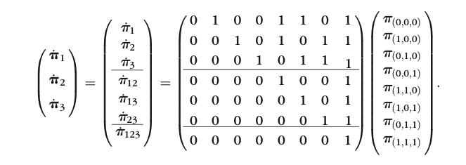
From Cai et al. (2006), p. 176
M2 Statistic
- The M2 statistic assesses model fit to univariate and bivariate marginal distributions of the data
- Both uni- and bivariate marginal distributions are subsumed into the MVB distribution
- In theory, M3, M4 and so on could be used
- The Cai et al. (2010) paper derives a sampling distribution for the M2 statistic
- This allows for the calculation of a p-value for the M2 statistic
- This is the most common method for assessing IRT model fit
- Other model fit measures can be constructed using this statistic
Ramifications of Limited Information Fit
- Despite the fact that the M2 statistic is a limited information fit statistic, it is still a global fit statistic
- But, it does not function entirely like the CFA-based versions
- If a model is judged to have adequate fit with M2, it does not mean the model fits the data absolutely
- It means the model fits the one- and two-way contingency tables of the data
- A model may not fit the higher order contingency tables of the data
- Model fit indices derived from M2 are not comparable to those derived from CFA-based methods
- This is because the target distributions are different
- Meaning: Commonly-used criteria for model fit are not applicable to IRT models
Local Misfit with Marginal and Bivariate statistics
Additionally, you can judge local misfit by examining the residuals of the marginal and bivariate statistics
- The residuals are the difference between the observed and expected frequencies
- You can create these using model statitics or posterior predictive distributions
- Mplus outputs these with the TECH10 option
- Alternatively, you can calculate summary statistics for bivariate tables and judge fit there:
- Tetrachoric correlations
- Kappas
Other Limited Information Fit Methods
Limited information estimation methods exist (lecture in two weeks)
- These use summary statistics of the data and apply CFA-like models to those statistics
- As such, all CFA-based model fit statistics are obtainable
- But, like M2, these may not have the same established criteria for model fit that CFA models have
Bayesian Model Fit
- Bayesian model fit is the process of assessing model fit using the posterior predictive distribution
- Overall idea: If a model fits the data well, then simulated data based on the model will resemble the observed data
- Ingredients in PPMC:
- Original data
- Typically characterized by some set of statistics (i.e, sample mean, standard deviation, covariance) applied to data
- Data simulated from posterior draws in the Markov Chain
- Summarized by the same set of statistics
- Original data
PPMC Process
The PPMC process is as follows
- Select parameters from a single (sampling) iteration of the Markov chain
- Using the selected parameters and the model, simulate a data set with the same size (number of observations/variables)
- From the simulated data set, calculate selected summary statistics (e.g. mean)
- Repeat steps 1-3 for a fixed number of iterations (perhaps across the whole chain)
- When done, compare position of observed summary statistics to that of the distribution of summary statitsics from simulated data sets (predictive distribution)
PPMC Charactaristics
PPMC methods are very useful
- They provide a visual way to determine if the model fits the observed data
- They are the main method of assessing absolute fit in Bayesian models
- Absolute fit assesses if a model fits the data
But, there are some drawbacks to PPMC methods
- Almost any statistic can be used
- Some are better than others
- No standard determining how much misfit is too much
- May be overwhelming to compute depending on your model
Posterior Predictive P-Values
We can quantify misfit from PPMC using a type of “p-value”
- The Posterior Predictive P-Value: The proportion of times the statistic from the simulated data exceeds that of the real data
- Useful to determine how far off a statistic is from its posterior predictive distribution
References for PPMC
You can read more about Bayesian PPMC from one of our recent graduates, Jihong Zhang:
- Local fit:
- Global Fit:
Relative Model Fit
Relative model fit is the process of determining which of a set of models fits the data best
- This is done by comparing the fit of the models to the data
- The best fitting model is the one that fits the data best
- Of note: all models being compared must have good absolute fit to the data
Relative Model Fit Methods
To compare the fit of two models, if the models are nested we can use the difference in the log-likelihoods of the models
- This is called the likelihood ratio test statistic
- The likelihood ratio test statistic is distributed as a Chi-square distribution with degrees of freedom equal to the difference in the number of parameters between the models
Relative Model Fit for Non-Nested or Bayesian Models
If the models are not nested, we can use the Information Criteria
- The Information Criteria are a set of model fit statistics that penalize models for having more parameters
- The most common are the AIC and BIC
- The model with the lowest AIC or BIC is the best fitting model
For Bayesian methods, analogus methods exist
- WAIC is the Wantanabe Akaike Information Criterion
- LOO-PSIS is the Leave-One-Out Pareto Smoothed Importance Sampling
- See the slides from my Bayesian class for more information
Wrapping Up
- Model fit is the process of determining whether the model is consistent with the data or whether one model is preferable to another
- Model fit is the first step in a validity argument
- Model fit methods are well-research but are seeminly rarely used in large-scale assessment (despite the high-stakes nature of the assessments)
Multidimensional Measurement Models (Fall 2023): Lecture 4