Relative model fit (depending on specific model comparions)
How to deal with multidimensionality
Removing misfitting items
Controlling for unwanted effects using auxiliary dimensions
Hoping dimensionality doesn’t matter (it does)
Lecture Overview
To describe what to do when multidimensionality is unwanted, we must first examine the types of MIRT models
Why: The nature of multidimensionality is important for determining what to do about it
When multidimensionality is unwanted, one remedy is ignoring it
Why: One type of multidimensionality is proportional to what a composite of unidimensional latent variables would look like
But, to get there, we must first dive into the models
Of note, the first section focuses largely on items that measure more than one dimension
This is where confusion often arises:
Most of the time, such cases are exploratory (although not always)
In such cases, these descriptive measures are seldom used, but they are used to help understand if a multidimensional model can be approximated well by a unidimensional model
Types of MIRT Models
A common classification of MIRT models is one of compensatory vs. non-compensatory models
Compensatory models allow for the effects of one dimension to be compensated for by the effects of another dimension
Example: A student who is low in math ability but high in reading ability may still be able to answer a math word problem correctly
Non-compensatory models do not allow for the effects of one dimension to be compensated for by the effects of another dimension
Example: A student who is low in math ability but high in reading ability may not be able to answer a math word problem correctly
Mathematical Distinctions of Compensatory vs. Non-Compensatory Models
Compensatory models are almost always the same form: additive within the space of the link function
For a binary item \(i\), measuring two dimensions \(\theta_1\) and \(\theta_2\), the probability of a correct response is: \[
P(Y_{pi} = 1 | \boldsymbol{\theta}_p) = \frac{\exp \left(\mu_i + \lambda_{i1} \theta_{p1} + \lambda_{i2} \theta_{p2} \right)}
{1+\exp \left(\mu_i + \lambda_{i1} \theta_{p1} + \lambda_{i2} \theta_{p2} \right)}
\]
What makes this model compensatory is due to the additive nature of the traits
Visualizing Compensatory Models
To show what a compensatory model looks like graphically, we can plot the item response function for a single item where:
\(\mu_i\) = -0.7$, \(\lambda_{i1}\) = 0.75$, \(\lambda_{i2}\) = 1.5$, and
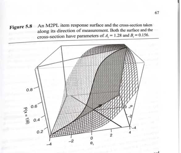
The term non-compensatory is used because a person cannot compensate for a deficiency in one dimension with a strength in another dimension
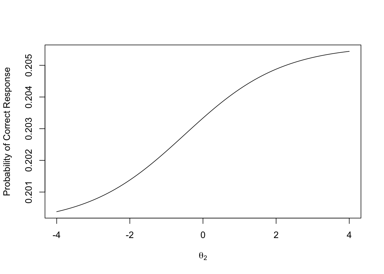
Here is a plot of the same model, but with \(\theta_1\) fixed at -4
Notice the range of the Y-axis–the maximum probability is 0.2054407
This occurs at \(\theta_2\) = 4
Another Way: Non-Compensatory Via Latent Variable Interactions
Here is the same contour plot, but with a latent variable interaction parameter
Descriptive Statistics of MIRT Models
For compensatory MIRT models, we can define some descriptive statistics that will help to show how a model functions
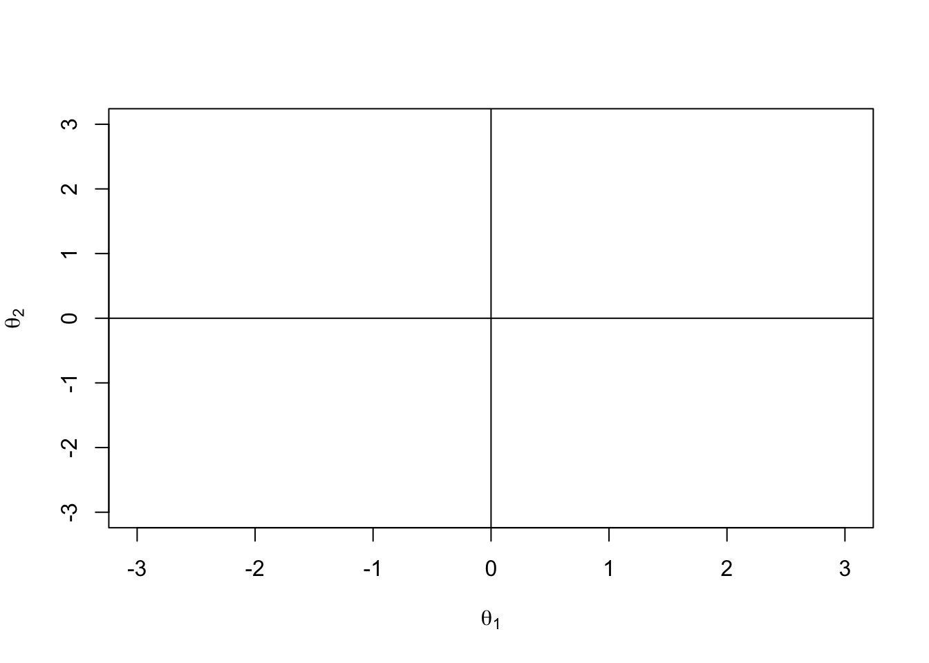
To do this, we must first define the \(\boldsymbol{\theta}\) space–the space of the latent variables
For simplicity, we will assume that \(E(\boldsymbol{\theta}) = \boldsymbol{0}\) and \(\text{diag}\left(Var(\boldsymbol{\theta})\right) = \text{diag}\left( \boldsymbol{I}\right)\)
For two dimensions, the \(\boldsymbol{\theta}\) space is:
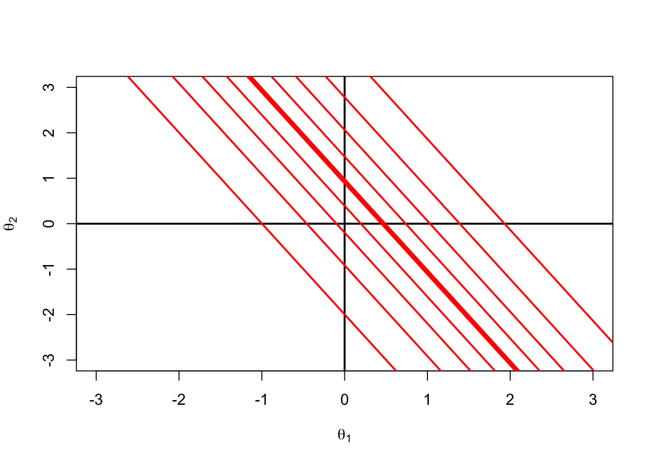
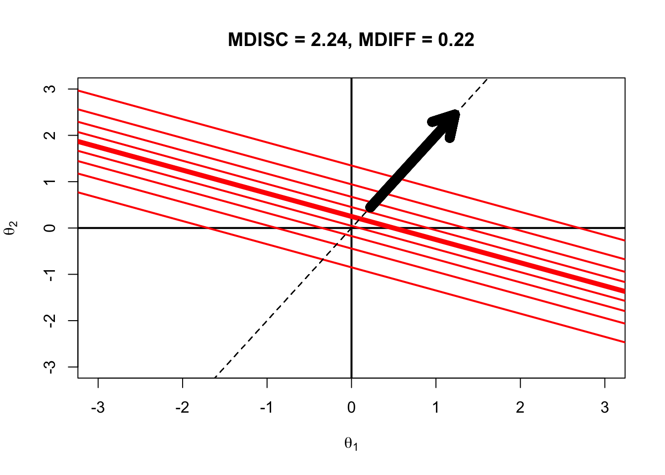
Theta Space: Contour Plot of MIRT ICC
Next, envision we have an item that measures two dimensions, \(\theta_1\) and \(\theta_2\)
We can then overlay the \(\boldsymbol{\theta}\) space with the equi-probablity contours of the item response function
This is called the Item Characteristic Curve (ICC)
The ICC is the probability of a correct response as a function of the latent variables
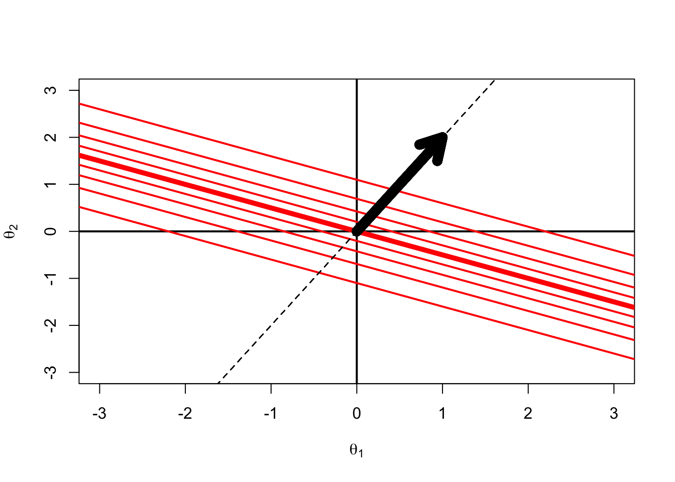
Direction of Steepest Slope: Direction of Measurement
A number of researchers (e.g., Muraki and Carlson, 1995, Reckase, 2009) define the direction of measurement as the direction of steepest slope of the ICC
We can show this direction with a dashed line in the plot
The slope of the dashed line comes from trigonometry and considers a triangle with sides \(\theta_1\) and \(\theta_2\)
Here, for a one unit change from the origin in \(\theta_1\) (or , \(\theta_1=1\)), we need the hypotenuse of the triangle formed by the line
But first, we need to describe the angle of the contours and the location of the 50% probability contour
Multidimensional Discrimination Index
The vector on the previous plot is oriented in the direction of measurement and has length proportional to the slope of the item in each direction (a “multidimensional slope”)
We can determine the length of the vector by using the Pythagorean Theorem
The length of the vector is the square root of the sum of the squares of the slopes in each direction
This is called the Multidimensional Discrimination Index (MDISC)
The “Direction of Measurement” (quotes used to denote a term that may not mean what it describes) is then the angle of the vector eminating from the origin in the direction of the steepest slope, relative to one dimension (here \(\theta_1\))
In radians: \[
\text{DOM}_i = \arccos \left( \frac{\lambda_{i1}}{MDISC_i} \right)
\]
This is the distance between the origin of the \(\boldsymbol{\theta}\)-space and the point where the direction of measurment intersects the 50% probability contour
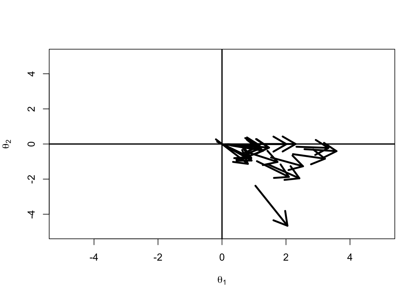
Multidimensional Difficulty Displayed
Vector Item Plots
We can use MDIFF and MDISC to plot items as vectors in two dimensions:
Later, we will see that this plot contributes to the “hope” solution of multidimensionality
Additional Information on MDISC and MDIFF
Wes Bonifay’s (2020) Sage book has a nice picture of a visual interpretation of MDISC and MDIFF
How to Detect Multidimensionality
As you are experiencing in HW4, there have been a number of methods developed to determine if an assessment is multidimensional
Principal components-based methods
PCA
Exploratory Factor Analysis Using Matrix Decompositions
ML-based Exploratory Factor Analysis
As we’ve seen, there is no such thing–only differing constraints
Note: no absolute model fit as all models will fit perfectly with full information model fit indices
Principal Components-Based Methods
PCA is a matrix decomposition method that finds the linear combination of variables that maximizes the variance
From matrix algebra, consider a square and symmetric matrix \(\boldsymbol{\Sigma}\) (e.g., a correlation or covariance matrix)
There exist a vector of eigenvalues \(\boldsymbol{\lambda}\) and a matrix of corresponding eigenvectors \(\boldsymbol{E}\) such that we can show that Sigma can be decomposed as:
We use the matrix of eigenvalues to help determine if a matrix is multidimensional
More PCA
The eigendecomposition (the factorization of a covariance or correlation matrix) of estimates the eigenvalues and eigenvectors using a closed form solution (called the characteristic polynomial)
The eigenvalues are the roots of the characteristic polynomial
The eigenvectors are the vectors that are unchanged by the transformation of the matrix
The eigenvectors are the directions of the principal components
The Components of PCA
The “components” are linear combinations of the variables that are uncorrelated and are ordered by the amount of variance they explain
The first component is the linear combination of variables that explains the most variance
The second component is the linear combination of variables that explains the second most variance, and so on
So, PCA is the process of developing hypothetical, uncorrelated, linear combinations of the data
One can almost envision why PCA gets used–sum scores
But, the components are not latent variables
And, the latent variables in latent variabel models don’t purport a sum
But, in the 1930s (and slightly before), this was the technology that was available
And, it is still used today
Factor analytic versions of PCA replace the diagonal of the covariance/correlation matrix with factor-analytic friendly terms (uniqueness)
Then does PCA
Many Issues with PCA
Solutions are widely unstable (sampling distributions of eigenvalues/eigenvectors are quite diffuse)
Not a good match to latent variable models directly
When data are not continuous (or plausibly continuous), Pearson correlation/covariance matrix is not appropriate
Missing data are an issue (assumed MCAR) as correlations pairwise delete missing data
Can you envision a method to fix some of these issues?
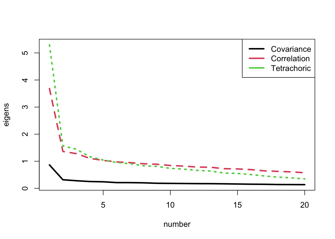
Conducting a PCA
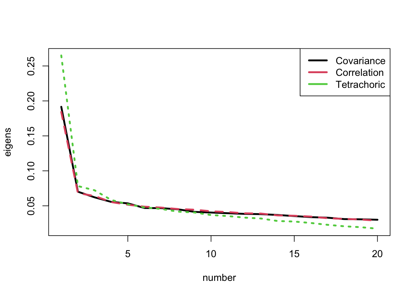
A PCA yields eigenvalues, which get used to describe how many “factors” are in the data
We then use the eigenvalues to determine how many factors to extract
A plot of the raw eigenvalues is given by the scree plot:
library(psych)
Attaching package: 'psych'
The following objects are masked from 'package:ggplot2':

    %+%, alpha
pearsonCovEigen =eigen(cov(mathData, use ="pairwise.complete.obs"))pearsonCorEigen =eigen(cor(mathData, use ="pairwise.complete.obs"))tetrachoricCorEigen =eigen(tetrachoric(mathData)$rho)
Removing misfitting items changes the meaning of the test (validity)
But, leaving them in changes makes the validity of the test questionable
To calculate model fit, item pairs need at least some observations on each
Linking designs may not permit model fit tests
Controlling for unwanted effects using auxiliary dimensions
Sometimes, multidimensionality may be caused by dimensions beyond ability
For example
If raters are providing data, there may be rater data
Items with a common stem may need a testlet effect
In such cases, adding non-reported dimensions to the psychometric model will control for the unwanted effects
But, estimation may be difficult
Marginalizing Over Unwanted Dimensions
A more recent method is to marginalize over unwanted dimensions:
A two-dimensional model is estimated
A single score is reported (integrate over the other score)
Reference: Ip, E. H., & Chen, S. H. (2014). Using projected locally dependent unidimensional models to measure multidimensional response data. In Handbook of Item Response Theory Modeling (pp. 226-251). Routledge.
Hoping Dimensionality Doesn’t Matter
Finally, what appears most common is to “hope” multidimensionality won’t greatly impact a unidimensional model
A unidimensional model fit to multidimensional data can have approximately good scores* if the vector plot has items in approximately the same direction
*Here, a score is a composite of scores across all dimensions
Reckase & Stout (1995) note a proof for “essential” unidimensionality
In such cases single scores may be a good reflection of multiple abilities
It appears we can now test this hypothesis via model comparisons with latent variable interaction models
Reckase MD, Stout W (1995) Conditions under which items that assess multiple abilities will be fit by unidimensional IRT models. Paper presented at the European meeting of the Psychometric Society, Leiden, The Netherlands
Wrapping Up
Today’s lecture was a lot! Here is a big-picture summary
Methods for detecting multidimensionality are numerous