Mixture Models and Latent Class Analysis
Lecture Outline
- Latent Class Analysis (LCA) Underlying theory (general contexts)
- Example analysis (and how to get estimates)
- Interpretation of model parameters
- Investigating model fit Extensions of the Technique: Latent Profile Analysis (LPA)
Clusters Versus Classes
- When a researcher mentions they are going to be using cluster analysis, they are most likely referring to one of the following:
- K-means clustering Hierarchical clustering using distance methods
- Discriminant analysis
- Taxometrics
- Much less often, latent class analysis is included in the group
- Although it too is useful for detecting clusters of observations
- For today’s lecture, we will consider clusters to be synonymous with classes
LCA Versus Other Methods
Although I am using the terms classes and clusters synonymously, the general approach of LCA differs from that of the other methods previously discussed
LCA is a model-based method for clustering (or classification)
- LCA fits a statistical model to the data in an attempt to determine classes
The other methods listed on the previous slide do not explicitly state a statistical model
By being model based, we are making very explicit assumptions about our data
- Assumptions that can be tested
Latent Class Analysis
LCA Introduction
- Latent class models are commonly attributed to Lazarsfeld and Henry (1968)
- The final number of classes is not usually predetermined prior to analysis with LCA
- The number of classes is determined through comparison of posterior fit statistics
- The characteristics of each class is also determined following the analysis
- Similar to K-means and hierarchical clustering techniques in this respect
Variable Types Used in LCA
- As it was originally conceived, LCA is an analysis that uses:
- A set of binary-outcome variables - values coded as zero or one
- Examples include:
- Test items - scored correct or incorrect
- True/false questions
- Gender
- Anything else that has two possible outcomes
LCA Process
- For a specified number of classes, LCA attempts to:
- For each class, estimate the probability that each variable is equal to one
- Estimate the probability that each observation falls into each class
- For each observation, the sum of these probabilities across classes equals one
- This is different from K-means where an observation is a member of a class with certainty
- Across all observations, estimate the probability that any observation falls into a class
LCA Estimation
- Estimation of LCA model parameters can be more complicated than other clustering methods:
- In hierarchical clustering, a search process is used with new distance matrices being created for each step
- K-means uses more of a brute-force approach - trying multiple random starting points then shifting cases between the different clusters until each is no longer shifted
- Both methods relied on distance metrics to find clustering solutions
- LCA estimation uses distributional assumptions to find classes
- The distributional assumptions provide the measure of “distance” in LCA
LCA Distributional Assumptions
- Because (for today) we have discussed LCA with binary-outcome variables, the distributional assumptions of LCA must use a binary-outcome distribution
- Within each latent class, the variables are assumed to:
- Be independent
- Be distributed marginally as Bernoulli:
- The Bernoulli distribution PMF is:
\[f(Y_{pi}) = \left(\pi_i \right)^{Y_{pi}} \left(1-\pi_i\right)^{(1-Y_{pi})}\]
- The Bernoulli distribution is a simple distribution for a single event - like flipping a coin
Bernoulli Distribution Illustration
- To illustrate the Bernoulli distribution (and statistical likelihoods in general), consider the following example
- To illustrate the Bernoulli distribution, consider a prediction of the result of the Northwester / Iowa football game as a binary-response item, \(Y\)
- Let’s say \(Y=1\) if Iowa wins, and \(Y=0\) if Northwestern wins
- My prediction is that Iowa has about an 87% chance of winning the game
- So, \(\pi=0.87\)
- Likewise, \(P(Y=1)=0.87\) and \(P(Y=0)=0.13\).
Bernoulli Distribution Illustration
The likelihood function for \(Y\) looks similar:
If \(Y=1\), the likelihood is: \[f(Y=1) = \left(0.87 \right)^{1} \left(1-0.87\right)^{(1-1)} =0.87\]
If \(Y=0\), the likelihood is: \[f(Y=0) = \left(0.87 \right)^{1} \left(1-0.87\right)^{(1-0)} =0.13\]
This example shows you how the likelihood function of a statistical distribution gives you the likelihood of an event occurring
In the case of discrete-outcome variables, the likelihood of an event is synonymous with the probability of the event occurring
Independent Bernoulli Variables
- To consider what independence of Bernoulli variables means, let’s consider the another game this season: Michigan v. Ohio State
- Let’s say we predict Michigan has a 57% chance of winning (or \(\pi_2=0.57\)).
- By assumption of independence of games, the probability of both Iowa and Michigan wining their games would be the product of the probability of winning each game separately:
\[P(Y_1=1,Y_2=1) = \pi_1 \pi_2 = 0.87 \times 0.57 = 0.4959\]
- More generally, we can express the likelihood of any set of occurrences by:
\[P(Y_1=y_1, Y_2=y_2,\ldots,Y_I=y_I) = \prod_{i=1}^{I} \pi_i^{Y_i}\left(1-\pi_i\right)^{\left(1-Y_i\right)}\]
Finite Mixture Models
Finite Mixture Models
- LCA models are special cases of more general models called Finite Mixture Models
- A finite mixture model expresses the distribution of a set of outcome variables, \(\boldsymbol{Y}\), as a function of the sum of weighted distribution likelihoods:
\[f(\textbf{Y}) = \sum_{c=1}^C \eta_c f(\textbf{Y}|c)\]
- With this general form we can now construct the (more specific) LCA model likelihood
- Here, we say that the conditional distribution of \(\boldsymbol{Y}\) given \(c\) is a set of independent Bernoulli variables
Latent Class Analysis as a FMM
A latent class model for the response vector of \(I\) variables (\(i =1,\ldots,I\)) with \(C\) classes (\(c=1,\ldots,C\)):
\[f(\boldsymbol{Y}_i) = \displaystyle {\sum_{c=1}^{C}\eta_c} \prod_{i=1}^{I} \pi_{ic}^{Y_{pi}}\left(1-\pi_{ic}\right)^{1-Y_{pi}}\]
Where:
- \(\eta_c\) is the probability that any individual is a member of class \(c\) (must sum to one)
- \(Y_{pi}\) is the observed response of person \(p\) to item \(i\)
- \(\pi_{ic}\) is the probability of a positive response to item \(i\) from an individual from class \(c\)
LCA Local Independence
- As shown in the LCA distributional form, LCA assumes all Bernoulli variables are independent given a class
- This assumption is called Local Independence
- It is also present in many other latent variable modeling techniques: Item response theory Factor analysis (with uncorrelated errors)
- What is implied is that any association between observed variables is accounted for only by the presence of the latent class
- Essentially, this is saying that the latent class is the reason that variables are correlated
Estimation Process
- Successfully applying an LCA model to data involves the resolution to two key questions:
- How many classes are present?
- What does each class represent?
- The answer to the first question comes from fitting LCA models with differing numbers of classes, then choosing the model with the best fit (to be defined later)
- The answer to the second question comes from inspecting the LCA model parameters of the solution that was deemed to have fit best
LCA Estimation Software
- There are several programs that exist that can estimate LCA models
- The package to be used today will be Mplus (with the Mixture add-on)
- Other packages also exist:
- Latent Gold
- A user-developed procedure in SAS (proc lca)
- Note: Due to the likelihood function not being unimodal (a single maximum), mixture models (and LCA models) are difficult to estimate using Bayesian methods
LCA Example #1
LCA Example #1
- To illustrate the process of LCA, we will use the example presented in Bartholomew and Knott (p. 142)
- The data are from a four-item test analyzed with an LCA by Macready and Dayton (1977)
- The test data used by Macready and Dayton were items from a math test
- Ultimately, Macready and Dayton wanted to see if examinees could be placed into two groups:
- Those who had mastered the material
- Those who had not mastered the material

LCA Example #1
LCA Example #1
- Several considerations will keep us from assessing the number of classes in Macready and Dayton’s data:
- We only have four items
- Macready and Dayton hypothesized two distinct classes: masters and non-masters
- For these reasons, we will only fit the two-class model and interpret the LCA model parameter estimates
Mplus Input
    TITLE:      LCA of Macready and Dayton's data (1977).
                Two classes.
    DATA:       FILE IS mddata.dat;
    VARIABLE:   NAMES ARE u1-u4;
                CLASSES = c(2);
                CATEGORICAL = u1-u4;
    ANALYSIS:   TYPE = MIXTURE;
                STARTS = 100 100;
    OUTPUT:     TECH1 TECH10;
    PLOT:       TYPE=PLOT3;
                SERIES IS u1(1) u2(2) u3(3) u4(4);
    SAVEDATA:   FORMAT IS f10.5;
                FILE IS examinee_ests.dat;
                SAVE = CPROBABILITIES;
LCA Parameter Information Types
- Recall, we have three pieces of information we can gain from an LCA:
- Sample information - proportion of people in each class (\(\eta_c\))
- Item information - probability of correct response for each item from examinees from each class (\(\pi_{ic}\))
- Examinee information - posterior probability of class membership for each examinee in each class (\(\alpha_{pc}\))
Estimates of \(\eta_c\) From Mplus:
    FINAL CLASS COUNTS AND PROPORTIONS FOR THE LATENT CLASSES
    BASED ON THE ESTIMATED MODEL

        Latent
       Classes

           1         83.29149          0.58656
           2         58.70851          0.41344
\(\eta_c\) are proportions in far right column
Estimates of \(\pi_{ic}\) From Mplus:
    RESULTS IN PROBABILITY SCALE
    Latent Class 1
     U1 Category 2         0.753    0.060
     U2 Category 2         0.780    0.069
     U3 Category 2         0.432    0.058
     U4 Category 2         0.708    0.063

    Latent Class 2
     U1 Category 2         0.209    0.066
     U2 Category 2         0.068    0.056
     U3 Category 2         0.018    0.037
     U4 Category 2         0.052    0.057
\(\pi_{ic}\) are proportions in left column, followed by asymptotic standard errors
Interpreting Classes
- After the analysis is finished, we need to examine the item probabilities to gain information about the characteristics of the classes
- An easy way to do this is to plot the item probabilities for each class
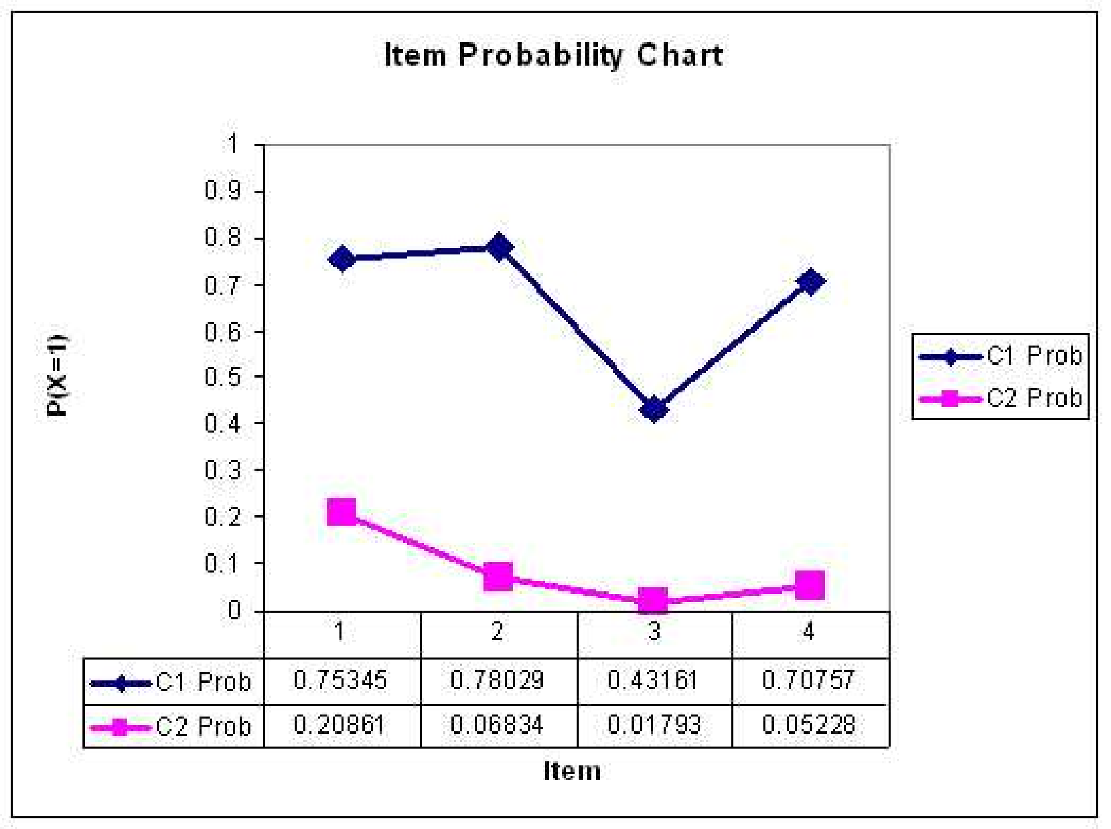
Interpreting Classes
- Here, we would say that Class 1 represents students who have mastered the material on the test
- We would say that Class 2 represents students who have not mastered the material on the test
Assessing Model Fit
Assessing Model Fit
- As with other statistical techniques, there is no one best way to assess the fit of an LCA model
- Techniques typically used can be put into several general categories:
- Model based hypothesis tests (absolute fit)
- Information criteria Measures based on distributional characteristics (for relative fit among a set of models)
- Entropy (depends on absolute fit)
Model Based Measures
- Recall the standard latent class model: A latent class model for the response vector of \(I\) variables (\(i =1,\ldots,I\)) with C classes (\(c=1,\ldots,C\)):
\[f(\boldsymbol{Y}_p) = \displaystyle {\sum_{c=1}^{C}\eta_c} \prod_{i=1}^{I} \pi_{ic}^{Y_{pi}} \left(1-\pi_{pi}\right)^{1-Y_{pi}}\]
- Model based measures of fit revolve around the model function listed above
- With just the function above, we can compute the probability of any given response pattern
- Mplus gives this information using the TECH10 output option
Model Chi-squared Test
- The \(\chi^2\) test compares the sets of response patterns that were observed with the set of response patterns expected under the model
- To form the \(\chi^2\) test, one must first compute the probability of each response pattern using the latent class model equation displayed on the last slide
- The hypothesis tested is that the observed frequency is equal to the expected frequency
- If the test has a low p-value, the model is said to not fit
- To demonstrate the model \(\chi^2\) test, let’s consider the results of the latent class model fit to the data from our running example (from Macready and Dayton, 1977)
Chi-squared Test Example
    Class Probabilities:
    Class   Probability
    1       0.587
    2       0.413

    Item Parameters
    class:         1
    item    prob    SE(prob)
    1       0.753   0.051
    2       0.780   0.051
    3       0.432   0.056
    4       0.708   0.054

    class:         2
    item    prob    SE(prob)
    1       0.209   0.060
    2       0.068   0.048
    3       0.018   0.029
    4       0.052   0.044
Chi-squared Test Example
- To begin, compute the probability of observing the pattern \([1 1 1 1]\)…
- Then, to find the expected frequency, multiply that probability by the number of observations in the sample
- Repeat that process for all cells…
- Then, compute \(\chi^2_p = \displaystyle \sum_r \frac{(O_r -E_r)^2}{E_r}\), where \(r\) represents each response pattern
- The degrees of freedom are equal to the number of response patterns minus model parameters minus one
- Then find the p-value, and decide if the model fits
Chi-squared from Mplus
         RESPONSE PATTERN FREQUENCIES AND CHI-SQUARE CONTRIBUTIONS

        Response          Frequency      Standard  Chi-square Contribution
         Pattern    Observed  Estimated  Residual  Pearson   Loglikelihood  Deleted
             1        41.00      41.04      0.01      0.00        -0.08
             2        13.00      12.91      0.03      0.00         0.18
             3         6.00       5.62      0.16      0.03         0.79
             4         7.00       8.92      0.66      0.41        -3.39
             5         1.00       1.30      0.27      0.07        -0.53
             6         3.00       1.93      0.77      0.59         2.63
             7         2.00       2.08      0.05      0.00        -0.15
             8         7.00       6.19      0.33      0.10         1.71
             9         4.00       4.04      0.02      0.00        -0.07
            10         6.00       6.13      0.05      0.00        -0.26
            11         5.00       6.61      0.64      0.39        -2.79
            12        23.00      19.74      0.79      0.54         7.04
            13         4.00       1.42      2.18      4.70         8.29
            14         1.00       4.22      1.59      2.46        -2.88
            15         4.00       4.90      0.41      0.16        -1.62
            16        15.00      14.95      0.01      0.00         0.09
Likelihood Ratio Chi-squared
The likelihood ratio Chi-square is a variant of the Pearson Chi-squared test, but still uses the observed and expected frequencies for each cell
The formula for this test is: \[G = 2 \sum_r O_r \ln\left(\frac{O_r}{E_r}\right)\]
The degrees of freedom are still the same as the Pearson Chi-squared test, however
Tests from Mplus
    Chi-Square Test of Model Fit for the Binary
    and Ordered Categorical (Ordinal) Outcomes

              Pearson Chi-Square

              Value                              9.459
              Degrees of Freedom                     6
              P-Value                           0.1494

              Likelihood Ratio Chi-Square

              Value                              8.966
              Degrees of Freedom                     6
              P-Value                           0.1755
Chi-squared Problems
- The Chi-square test is reasonable for situations where the sample size is large, and the number of variables is small
- If there are too many cells where the observed frequency is small (or zero), the test is not valid
- Note that the total number of response patterns in an LCA is \(2^I\), where \(I\) is the total number of variables
- For our example, we had four variables, so there were 16 possible response patterns
- If we had 20 variables, there would be a total of 1,048,576 response patterns
- Think about the number of observations you would have to have if you were to observe at least one person with each response pattern
- Now think about if the items were highly associated (you would need even more people)
Model Comparison
- So, if model-based Chi-squared tests are valid only for a limited set of analyses, what else can be done?
- One thing is to look at comparative measures of model fit
- Such measures will allow the user to compare the fit of one solution (say two classes) to the fit of another (say three classes)
- Note that such measures are only valid as a means of relative model fit - what do these measures become if the model fits perfectly?
Log Likelihood
- Prior to discussing anything, let’s look at the log-likelihood function, taken across all the observations in our data set
- The log likelihood serves as the basis for the AIC and BIC, and is what is maximized by the estimation algorithm
- The likelihood function is the model formulation across the joint distribution of the data (all observations):
\[L(\boldsymbol{Y}_p) =\prod_{p=1}^N \left[\displaystyle {\sum_{c=1}^{C}\eta_c} \prod_{i=1}^{I} \pi_{ic}^{Y_{pi}} \left(1-\pi_{pi}\right)^{1-Y_{pi}} \right]\]
Log Likelihood
- The log likelihood function is the log of the model formulation across the joint distribution of the data (all observations):
\[Log L(\boldsymbol{Y}_{pi}) =\log \left(\prod_{p=1}^N \left[\displaystyle {\sum_{c=1}^{C}\eta_c} \prod_{i=1}^{I} \pi_{ic}^{Y_{pi}} \left(1-\pi_{pi}\right)^{1-Y_{pi}} \right]\right)\]
\[Log L(\boldsymbol{Y}_{pi}) = \sum_{p=1}^N \log \left( \displaystyle {\sum_{c=1}^{C}\eta_c} \prod_{i=1}^{I} \pi_{ic}^{Y_{pi}} \left(1-\pi_{pi}\right)^{1-Y_{pi}}\right)\]
Here, the log function taken is typically base \(e\) - the natural log
The log likelihood is a function of the observed responses for each person and the model parameters
Information Criteria
- The Akaike Information Criterion (AIC) is a measure of the goodness of fit of a model that considers the number of model parameters (q)
\[AIC = 2q - 2 \log L\]
- Schwarz’s Information Criterion (also called the Bayesian Information Criterion or the Schwarz-Bayesian Information Criterion) is a measure of the goodness of fit of a model that considers the number of parameters (q) and the number of observations (N):
\[BIC = q \log (N) - 2 \log L\]
Fit from Mplus
    TESTS OF MODEL FIT

    Loglikelihood

              H0 Value                        -331.764

    Information Criteria

              Number of Free Parameters              9
              Akaike (AIC)                     681.527
              Bayesian (BIC)                   708.130
              Sample-Size Adjusted BIC         679.653
                (n* = (n + 2) / 24)
              Entropy                            0.754
Information Criteria
- When considering which model “fits” the data best, the model with the lowest AIC or BIC should be considered
- Although AIC and BIC are based on good statistical theory, neither is a gold standard for assessing which model should be chosen
- Furthermore, neither will tell you, overall, if your model estimates bear any decent resemblance to your data
- You could be choosing between two (equally) poor models - other measures are needed
Distributional Measures of Model Fit
- The model-based Chi-squared provided a measure of model fit, while narrow in the times it could be applied, that tried to map what the model said the data looked like to what the data actually looked like
- The same concept lies behind the ideas of distributional measures of model fit - use the parameters of the model to “predict” what the data should look like
- In this case, measures that are easy to attain are measures that look at:
- Each variable marginally - the mean (or proportion)
- The bivariate distribution of each pair of variables - contingency tables (for categorical variables), correlation
- matrices, or covariance matrices
Marginal Measures
- For each item, the model-predicted mean of the item (proportion of people responding with a value of one) is given by:
\[\hat{\bar{Y}}_i = \hat{E}(Y_i) = \sum_{c=1}^J \hat{\eta}_c \times \hat{\pi}_{ic}\]
Across all items, you can then form an aggregate measure of model fit by comparing the observed mean of the item to that found under the model, such as the root mean squared error (note: this is not RMSEA from CFA/IFA): \[RMSE = \sqrt{\frac{\sum_{i=1}^I(\hat{\bar{Y}}_i - \bar{Y}_i)^2}{I}}\]
Often, there is not much difference between observed and predicted mean (depending on the model, the fit will always be perfect)
Marginal Measures from Mplus From Mplus (using TECH10):
         UNIVARIATE MODEL FIT INFORMATION

                                   Estimated Probabilities
         Variable              H1           H0    Standard Residual
         U1
           Category 1        0.472        0.472         0.000
           Category 2        0.528        0.528         0.000
         U2
           Category 1        0.514        0.514         0.000
           Category 2        0.486        0.486         0.000
         U3
           Category 1        0.739        0.739         0.000
           Category 2        0.261        0.261         0.000
         U4
           Category 1        0.563        0.563         0.000
           Category 2        0.437        0.437         0.000
Bivariate Measures
- For a pair of items (say \(a\) and \(b\), the model-predicted probability of both being one is given in the same way:
\[\hat{P}(Y_a = 1, Y_b=1) = \sum_{c=1}^C \hat{\eta}_c \times \hat{\pi}_{ac} \times \hat{\pi}_{bc}\]
- Given the marginal means, you can now form a 2 x 2 table of the probability of finding a given pair of responses to variable \(a\) and \(b\)
Bivariate Measures
- Given the model-predicted contingency table (on the last slide) for every pair of items, you can then form a measure of association for the items
- There are multiple ways to summarize association in a contingency table
- Depending on your preference, you could use:
- Pearson correlation
- Tetrachoric correlation
- Cohen’s kappa
- After that, you could then summarize the discrepancy between what your model predicts and what you have observed in the data
- Such as the RMSE, MAD, or BIAS
Bivariate Measures from Mplus From Mplus (using TECH10):
         BIVARIATE MODEL FIT INFORMATION

                                                  Estimated Probabilities
         Variable       Variable              H1           H0     Standard Residual
         U1             U2
           Category 1     Category 1        0.352        0.337         0.391
           Category 1     Category 2        0.120        0.135        -0.540
           Category 2     Category 1        0.162        0.177        -0.483
           Category 2     Category 2        0.366        0.351         0.387
Entropy
- The entropy of a model is defined to be a measure of classification uncertainty
- To define the entropy of a model, we must first look at the posterior probability of class membership, let’s call this \(\hat{\alpha}_{ic}\)
- Here, \(\hat{\alpha}_{ic}\) is the estimated probability that observation \(i\) is a member of class \(c\)
- The entropy of a model is defined as:
\[EN(\boldsymbol{\alpha}) = - \sum_{i=1}^N \sum_{c=1}^C \hat{\alpha}_{ic} \log \hat{\alpha}_{ic}\]
Relative Entropy
The entropy equation on the last slide is bounded from \([0,\infty)\), with higher values indicated a larger amount of uncertainty in classification
Mplus reports the relative entropy of a model, which is a rescaled version of entropy:
\[E = 1 - \frac{EN(\boldsymbol{\alpha})}{N \log C}\]
The relative entropy is defined on \([0,1]\), with values near one indicating high certainty in classification and values near zero indicating low certainty
Fit from Mplus
    TESTS OF MODEL FIT

    Loglikelihood

              H0 Value                        -331.764

    Information Criteria

              Number of Free Parameters              9
              Akaike (AIC)                     681.527
              Bayesian (BIC)                   708.130
              Sample-Size Adjusted BIC         679.653
                (n* = (n + 2) / 24)
              Entropy                            0.754
From LCA to More Useful FMMs
General Notational Framework
The finite mixture model is a general framework for modeling data that can be expressed as:
\[f(\boldsymbol{Y}) = \sum_{c=1}^C \eta_c f(\boldsymbol{Y}|c)\]
- Where \(\boldsymbol{Y}\) is a vector of observed variables
- \(f(\boldsymbol{Y})\) is the joint distribution of the observed variables
- \(f(\boldsymbol{Y}|c)\) is the conditional distribution of the observed variables given class \(c\)
- The distributional form of \(f(\boldsymbol{Y}|c)\) is dependent on the type of observed variables
- \(\eta_c\) is the probability of class membership for class \(c\)
- \(C\) is the number of classes
Mixture IRT Models
- Perhaps most relevant to this class is are the family of models that go by the term “Mixture Item Response Models”
- Most popular: Mixture Rasch Models
- The general form of a mixture IRT model for binary items is:
\[f(\boldsymbol{Y}_p \mid \theta_p) = \sum_{c=1}^C \eta_c f(\boldsymbol{Y}_p|c, \theta_p)\]
Where:
\[f(\boldsymbol{Y}|c) = \prod_{i=1}^I \pi_{ic}^{Y_{pi}} \left( 1-\pi_{ic} \right)^{1-Y_{pi}}\]
And:
\[\pi_{ic} = P \left( Y_{pi} = 1 \mid \theta_p \right) = \frac{\exp \left( a_{ic} \left( \theta_p - b_{ic}\right) \right)}{1+\exp \left( a_{ic} \left( \theta_p - b_{ic}\right) \right)}\]
Mixture IRT Model Parameters
- The parameters of a mixture IRT model are:
- \(\eta_c\) - the probability of class membership for class \(c\)
- \(a_{ic}\) - the discrimination parameter for item \(i\) in class \(c\)
- \(b_{ic}\) - the difficulty parameter for item \(i\) in class \(c\)
Mixture IRT Model Motivation
- Here, several researchers had the belief that mixture IRT models would reveal differing strategies used by examinees on items
- But, that’s assuming that the classes are meaningful
- In Templin and Alexeev (2011), we showed that classes were often formed when a single-class IRT model misfit the data
- Classes can be spurious
Latent Class Analysis: Wrap Up
LCA Limitations
- LCA has limitations which can make its general application difficult:
- Classes not known prior to analysis
- Class characteristics not know until after analysis
- Both of these problems are related to LCA being an exploratory procedure for understanding data
- Diagnostic Classification Models can be thought of as one type of a confirmatory LCA
- By placing constraints on the class item probabilities and specifying what our classes mean prior to analysis
LCA Summary
- Latent class analysis is a model-based technique for finding clusters in binary (categorical) data
- Each of the variables is assumed to:
- Have a Bernoulli distribution
- Be independent given class
- Additional reading (book): Lazarsfeld and Henry (1968). Latent structure analysis
Multidimensional Measurement Models (Fall 2023): Lecture 10