The Educational Measurement Problem: Total vs. Subscores
The issue (from K-12 assessment):
Assessment programs are designed to provide a single score for each student for each subject (e.g., reading, math, science, etc.)
However, many states also wish to provide more detailed information to each student
“Subscores” are often used to provide more detailed information about a student’s performance
A subscore is a score that is based on a subset of the items on a test
For example, a reading test may have a subscore for “vocabulary” and a subscore for “reading comprehension”
A math test may have a subscore for “algebra” and a subscore for “geometry”
The problem with subscores when having a unidimensional total score
The basic problem is a modeling problem:
The total score has a unidimensional model
The subscores have a multidimensional model
The two models are incompatible and cannot both be correct
Unidimensional Model
The model for the total score is often a unidimensional model:
\[
P(Y_{pi} = 1 | \theta_p) =
\frac{\exp \left(a_i \left( \theta_p - b_i \right) \right)}
{1 + \exp \left(a_i \left( \theta_p - b_i \right) \right)}
\]
This model applies for all items \(i\) and all persons \(p\)
Note: The model shown is a two-parameter IRT model, but in general, there will be one latent variable in a unidimensional model
# format data = temp$ responseMatrix= temp$ Qmatrix= Qmatrix[which (rownames (Qmatrix) %in% paste0 ("item" , 11 : 30 )), ]= reducedQ[, which (colSums (reducedQ) > 0 )]# using only Algebra items (11:30) ==================================================================================== = responseMatrix[paste0 ("item" , 11 : 30 )]# remove cases that are all NA ======================================================================================== = dataMat[apply (dataMat, 1 , function (x) ! all (is.na (x))), ]# create lavaan model for unidimensional model ======================================================================== names (responseMatrix)
 [1] "item1"           "item2"           "item3"           "item4"
 [5] "item5"           "item6"           "item7"           "item8"
 [9] "item9"           "item10"          "item11"          "item12"
[13] "item13"          "item14"          "item15"          "item16"
[17] "item17"          "item18"          "item19"          "item20"
[21] "item21"          "item22"          "item23"          "item24"
[25] "item25"          "item26"          "item27"          "item28"
[29] "item29"          "item30"          "item31"          "item32"
[33] "item33"          "item34"          "item35"          "item36"
[37] "item37"          "item38"          "item39"          "item40"
[41] "item41"          "item42"          "item43"          "item44"
[45] "item45"          "item46"          "item47"          "item48"
[49] "item49"          "item50"          "courseNameCombo" "id"
= " theta =~ item11 + item12 + item13 + item14 + item15 + item16 + item17 + item18 + item19 + item20 + item21 + item22 + item23 + item24 + item25 + item26 + item27 + item28 + item29 + item30 " = cfa (model = unidimensionalModel_syntax, data = responseMatrix, estimator = "WLSMV" , ordered = paste0 ("item" , 11 : 30 ), std.lv = TRUE , parameterization = "theta" summary (unidimensionalModel, fit.measures = TRUE , standardized = TRUE )
lavaan 0.6.15 ended normally after 15 iterations
Estimator DWLS
Optimization method NLMINB
Number of model parameters 40
Used Total
Number of observations 1099 2541
Model Test User Model:
Standard Scaled
Test Statistic 419.002 514.212
Degrees of freedom 170 170
P-value (Chi-square) 0.000 0.000
Scaling correction factor 0.847
Shift parameter 19.655
simple second-order correction
Model Test Baseline Model:
Test statistic 5341.853 3322.839
Degrees of freedom 190 190
P-value 0.000 0.000
Scaling correction factor 1.644
User Model versus Baseline Model:
Comparative Fit Index (CFI) 0.952 0.890
Tucker-Lewis Index (TLI) 0.946 0.877
Robust Comparative Fit Index (CFI) 0.799
Robust Tucker-Lewis Index (TLI) 0.775
Root Mean Square Error of Approximation:
RMSEA 0.037 0.043
90 Percent confidence interval - lower 0.032 0.039
90 Percent confidence interval - upper 0.041 0.047
P-value H_0: RMSEA <= 0.050 1.000 0.997
P-value H_0: RMSEA >= 0.080 0.000 0.000
Robust RMSEA 0.073
90 Percent confidence interval - lower 0.065
90 Percent confidence interval - upper 0.080
P-value H_0: Robust RMSEA <= 0.050 0.000
P-value H_0: Robust RMSEA >= 0.080 0.061
Standardized Root Mean Square Residual:
SRMR 0.066 0.066
Parameter Estimates:
Standard errors Robust.sem
Information Expected
Information saturated (h1) model Unstructured
Latent Variables:
Estimate Std.Err z-value P(>|z|) Std.lv Std.all
theta =~
item11 0.864 0.074 11.634 0.000 0.864 0.654
item12 0.286 0.053 5.421 0.000 0.286 0.275
item13 0.768 0.062 12.382 0.000 0.768 0.609
item14 0.589 0.053 11.017 0.000 0.589 0.508
item15 0.474 0.049 9.626 0.000 0.474 0.428
item16 0.703 0.055 12.835 0.000 0.703 0.575
item17 0.710 0.056 12.576 0.000 0.710 0.579
item18 0.867 0.066 13.192 0.000 0.867 0.655
item19 0.912 0.067 13.547 0.000 0.912 0.674
item20 0.820 0.078 10.577 0.000 0.820 0.634
item21 0.173 0.045 3.799 0.000 0.173 0.170
item22 0.310 0.057 5.441 0.000 0.310 0.296
item23 0.437 0.056 7.736 0.000 0.437 0.400
item24 0.374 0.052 7.164 0.000 0.374 0.350
item25 0.433 0.053 8.129 0.000 0.433 0.398
item26 0.569 0.062 9.150 0.000 0.569 0.494
item27 0.422 0.048 8.785 0.000 0.422 0.389
item28 0.605 0.057 10.706 0.000 0.605 0.518
item29 0.257 0.058 4.411 0.000 0.257 0.249
item30 0.390 0.053 7.292 0.000 0.390 0.363
Intercepts:
Estimate Std.Err z-value P(>|z|) Std.lv Std.all
.item11 0.000 0.000 0.000
.item12 0.000 0.000 0.000
.item13 0.000 0.000 0.000
.item14 0.000 0.000 0.000
.item15 0.000 0.000 0.000
.item16 0.000 0.000 0.000
.item17 0.000 0.000 0.000
.item18 0.000 0.000 0.000
.item19 0.000 0.000 0.000
.item20 0.000 0.000 0.000
.item21 0.000 0.000 0.000
.item22 0.000 0.000 0.000
.item23 0.000 0.000 0.000
.item24 0.000 0.000 0.000
.item25 0.000 0.000 0.000
.item26 0.000 0.000 0.000
.item27 0.000 0.000 0.000
.item28 0.000 0.000 0.000
.item29 0.000 0.000 0.000
.item30 0.000 0.000 0.000
theta 0.000 0.000 0.000
Thresholds:
Estimate Std.Err z-value P(>|z|) Std.lv Std.all
item11|t1 0.460 0.055 8.384 0.000 0.460 0.348
item12|t1 0.645 0.043 14.979 0.000 0.645 0.620
item13|t1 0.128 0.048 2.654 0.008 0.128 0.102
item14|t1 0.131 0.044 2.966 0.003 0.131 0.113
item15|t1 0.082 0.042 1.955 0.051 0.082 0.074
item16|t1 -0.141 0.046 -3.060 0.002 -0.141 -0.115
item17|t1 -0.038 0.046 -0.815 0.415 -0.038 -0.031
item18|t1 -0.044 0.050 -0.877 0.381 -0.044 -0.033
item19|t1 -0.113 0.051 -2.214 0.027 -0.113 -0.083
item20|t1 0.610 0.057 10.675 0.000 0.610 0.472
item21|t1 0.266 0.039 6.824 0.000 0.266 0.262
item22|t1 0.824 0.046 17.874 0.000 0.824 0.787
item23|t1 0.623 0.046 13.661 0.000 0.623 0.571
item24|t1 0.512 0.043 11.893 0.000 0.512 0.480
item25|t1 0.484 0.044 11.049 0.000 0.484 0.444
item26|t1 0.618 0.049 12.572 0.000 0.618 0.537
item27|t1 0.170 0.041 4.109 0.000 0.170 0.157
item28|t1 0.345 0.046 7.485 0.000 0.345 0.295
item29|t1 0.781 0.045 17.458 0.000 0.781 0.756
item30|t1 0.551 0.044 12.571 0.000 0.551 0.513
Variances:
Estimate Std.Err z-value P(>|z|) Std.lv Std.all
.item11 1.000 1.000 0.572
.item12 1.000 1.000 0.925
.item13 1.000 1.000 0.629
.item14 1.000 1.000 0.742
.item15 1.000 1.000 0.817
.item16 1.000 1.000 0.669
.item17 1.000 1.000 0.665
.item18 1.000 1.000 0.571
.item19 1.000 1.000 0.546
.item20 1.000 1.000 0.598
.item21 1.000 1.000 0.971
.item22 1.000 1.000 0.912
.item23 1.000 1.000 0.840
.item24 1.000 1.000 0.877
.item25 1.000 1.000 0.842
.item26 1.000 1.000 0.755
.item27 1.000 1.000 0.849
.item28 1.000 1.000 0.732
.item29 1.000 1.000 0.938
.item30 1.000 1.000 0.868
theta 1.000 1.000 1.000
Scales y*:
Estimate Std.Err z-value P(>|z|) Std.lv Std.all
item11 0.757 0.757 1.000
item12 0.962 0.962 1.000
item13 0.793 0.793 1.000
item14 0.862 0.862 1.000
item15 0.904 0.904 1.000
item16 0.818 0.818 1.000
item17 0.816 0.816 1.000
item18 0.756 0.756 1.000
item19 0.739 0.739 1.000
item20 0.773 0.773 1.000
item21 0.985 0.985 1.000
item22 0.955 0.955 1.000
item23 0.916 0.916 1.000
item24 0.937 0.937 1.000
item25 0.918 0.918 1.000
item26 0.869 0.869 1.000
item27 0.921 0.921 1.000
item28 0.856 0.856 1.000
item29 0.969 0.969 1.000
item30 0.932 0.932 1.000
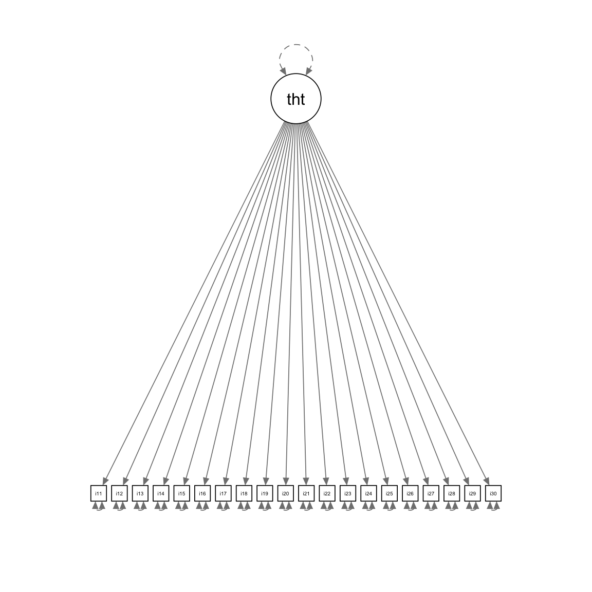
= lavPredict (unidimensionalModel):: semPaths (unidimensionalModel, sizeMan = 2.5 , style = "mx" , intercepts = FALSE , thresholds = FALSE )
Unidimensional Model Path Diagram
:: semPaths (unidimensionalModel, sizeMan = 2.5 , style = "mx" , intercepts = FALSE , thresholds = FALSE )
Common Subscore Estimation Methods
With an overall score from the unidimensional model, often subscores are formed by one of the following methods:
Using the unidimensional model parameters to create IRT-based subscores where:
Each score is a latent variable estimate from the IRT model
Each estimate is with respect to only the set of items that contribute/measure the subdomains
Summing items that measure the subdomains (here, the standards)
Lecture 13 showed this was a parallel items model
Each of these methods has problems (to be discussed)
Unidimensional IRT-Model Based Subscores
Unidimensional IRT-Model Subscores are created by:
Taking the estimated parameters of only the items measuring a subdomain
Using IRT-based scoring methods
Note: As I am using lavaan for this lecture, I cannot easily create these scores
Instead: Showing a simulation with the mirt package
See file subscoreSame.R for methods for constructing scores
Sum-score Based Subscores
Sum-score based subscores are estimated by summing the items that measure each subdomain
= Qmatrix[which (rownames (Qmatrix) %in% paste0 ("item" , 11 : 30 )), ]= reducedQ[, which (colSums (reducedQ) > 0 )]= as.matrix (dataMat) %*% as.matrix (reducedQ)# problem with sumscores: missing data head (sumScores)
   A.REI.1 A.REI.2 A.REI.8 A.CED.2
1        2       5       0       1
2        3       0       0       1
4        2       1       1       2
7        1       2       1       0
9        4       1       2       0
11       3       4       4       4
Sum-score Based Subscores: Missing Data
One problem with sum-score based subscores is missing data
If a person omits a response, their total score possible is lower
Solution: Mean-based Subscores (the mean of all items administered)
# resolution: make an average score for each student = nItems = matrix (0 , nrow = nrow (sumScores), ncol = ncol (sumScores))for (person in 1 : nrow (dataMat)){for (col in 1 : ncol (reducedQ)){for (row in 1 : nrow (reducedQ)){if (reducedQ[row, col] == 1 && ! is.na (dataMat[person, row])){= averageScores[person, col] + dataMat[person, row]= nItems[person, col] + 1 = averageScores[person, col] / nItems[person, col]head (averageScores)
     [,1] [,2] [,3] [,4]
[1,]  0.4  1.0  0.0  0.2
[2,]  0.6  0.0  0.0  0.2
[3,]  0.4  0.2  0.2  0.4
[4,]  0.2  0.4  0.2  0.0
[5,]  0.8  0.2  0.4  0.0
[6,]  0.6  0.8  0.8  0.8
Plots of Subscores vs. Overall Score
# plotting scores: par (mfrow = c (2 , 2 ))for (standard in 1 : ncol (reducedQ)){plot (x = sumScores[,standard], y = unidimensionalScores, main = "Sum Scores vs. Unidimensional Scores" , ylab = "IRT Total Theta" ,xlab = paste0 ("Sum Score " , colnames (reducedQ)[standard]))
Measurement Model Implied by Sumscore-based Subscores
The measurement model implied by sumscore-based subscores is a multidimensional CFA model where:
Each item intercept, loading, and unique variance are constrained to be equal across subdomains
The correlation between factors is fixed to zero
Subscore 1: \[
\begin{array}{c}
Y_{p1} = \mu_1 + \lambda_1 F_{p1} + e_{p1}; e_{p1} \sim N(0, \psi^2_1) \\
Y_{p2} = \mu_2 + \lambda_1 F_{p1} + e_{p2}; e_{p2} \sim N(0, \psi^2_1) \\
\vdots \\
Y_{p5} = \mu_5 + \lambda_1 F_{p1} + e_{p5}; e_{p5} \sim N(0, \psi^2_1)
\end{array}
\]
Subscore 2: \[
\begin{array}{c}
Y_{p6} = \mu_6 + \lambda_2 F_{p2} + e_{p6}; e_{p6} \sim N(0, \psi^2_2) \\
Y_{p7} = \mu_7 + \lambda_2 F_{p2} + e_{p7}; e_{p7} \sim N(0, \psi^2_2) \\
\vdots \\
Y_{p10} = \mu_10 + \lambda_2 F_{p2} + e_{p10}; e_{p10} \sim N(0, \psi^2_2)
\end{array}
\]
Structural model:
\[
\begin{bmatrix}
\theta_{p1} \\
\theta_{p2} \\
\theta_{p3} \\
\theta_{p4} \\
\end{bmatrix}
\sim N \left(\boldsymbol{0}, \boldsymbol{I}_{4} \right)
\]
Implementing Sumscore-Based Subscore Model in lavaan
= " # constrain all loadings to be equal within each subscore theta1 =~ L1*item11 + L1*item12 + L1*item13 + L1*item14 + L1*item15 theta2 =~ L2*item16 + L2*item17 + L2*item18 + L2*item19 + L2*item20 theta3 =~ L3*item21 + L3*item22 + L3*item23 + L3*item24 + L3*item25 theta4 =~ L4*item26 + L4*item27 + L4*item28 + L4*item29 + L4*item30 # set the unique variances to be equal within each subscore item11 ~~ U1*item11; item12 ~~ U1*item12; item13 ~~ U1*item13; item14 ~~ U1*item14; item15 ~~ U1*item15; item16 ~~ U2*item16; item17 ~~ U2*item17; item18 ~~ U2*item18; item19 ~~ U2*item19; item20 ~~ U2*item20; item21 ~~ U3*item21; item22 ~~ U3*item22; item23 ~~ U3*item23; item24 ~~ U3*item24; item25 ~~ U3*item25; item26 ~~ U4*item26; item27 ~~ U4*item27; item28 ~~ U4*item28; item29 ~~ U4*item29; item30 ~~ U4*item30; # set all covariances to zero theta1 ~~ 0*theta2 theta1 ~~ 0*theta3 theta1 ~~ 0*theta4 theta2 ~~ 0*theta3 theta2 ~~ 0*theta4 theta3 ~~ 0*theta4 " = cfa (model = parallelItems_syntax, data = dataMat, estimator = "MLR" ,std.lv = TRUE , summary (parallelItemsModel, fit.measures = TRUE , standardized = TRUE )
lavaan 0.6.15 ended normally after 17 iterations

  Estimator                                         ML
  Optimization method                           NLMINB
  Number of model parameters                        40
  Number of equality constraints                    32

  Number of observations                          1099

Model Test User Model:
                                              Standard      Scaled
  Test Statistic                              1189.531    1236.996
  Degrees of freedom                               202         202
  P-value (Chi-square)                           0.000       0.000
  Scaling correction factor                                  0.962
    Yuan-Bentler correction (Mplus variant)

Model Test Baseline Model:

  Test statistic                              2354.623    2286.856
  Degrees of freedom                               190         190
  P-value                                        0.000       0.000
  Scaling correction factor                                  1.030

User Model versus Baseline Model:

  Comparative Fit Index (CFI)                    0.544       0.506
  Tucker-Lewis Index (TLI)                       0.571       0.536

  Robust Comparative Fit Index (CFI)                         0.539
  Robust Tucker-Lewis Index (TLI)                            0.566

Loglikelihood and Information Criteria:

  Loglikelihood user model (H0)             -14167.940  -14167.940
  Scaling correction factor                                  0.158
      for the MLR correction
  Loglikelihood unrestricted model (H1)     -13573.174  -13573.174
  Scaling correction factor                                  0.955
      for the MLR correction

  Akaike (AIC)                               28351.879   28351.879
  Bayesian (BIC)                             28391.896   28391.896
  Sample-size adjusted Bayesian (SABIC)      28366.487   28366.487

Root Mean Square Error of Approximation:

  RMSEA                                          0.067       0.068
  90 Percent confidence interval - lower         0.063       0.065
  90 Percent confidence interval - upper         0.070       0.072
  P-value H_0: RMSEA <= 0.050                    0.000       0.000
  P-value H_0: RMSEA >= 0.080                    0.000       0.000

  Robust RMSEA                                               0.067
  90 Percent confidence interval - lower                     0.063
  90 Percent confidence interval - upper                     0.071
  P-value H_0: Robust RMSEA <= 0.050                         0.000
  P-value H_0: Robust RMSEA >= 0.080                         0.000

Standardized Root Mean Square Residual:

  SRMR                                           0.119       0.119

Parameter Estimates:

  Standard errors                             Sandwich
  Information bread                           Observed
  Observed information based on                Hessian

Latent Variables:
                   Estimate  Std.Err  z-value  P(>|z|)   Std.lv  Std.all
  theta1 =~
    item11    (L1)    0.207    0.008   25.443    0.000    0.207    0.428
    item12    (L1)    0.207    0.008   25.443    0.000    0.207    0.428
    item13    (L1)    0.207    0.008   25.443    0.000    0.207    0.428
    item14    (L1)    0.207    0.008   25.443    0.000    0.207    0.428
    item15    (L1)    0.207    0.008   25.443    0.000    0.207    0.428
  theta2 =~
    item16    (L2)    0.267    0.007   39.947    0.000    0.267    0.542
    item17    (L2)    0.267    0.007   39.947    0.000    0.267    0.542
    item18    (L2)    0.267    0.007   39.947    0.000    0.267    0.542
    item19    (L2)    0.267    0.007   39.947    0.000    0.267    0.542
    item20    (L2)    0.267    0.007   39.947    0.000    0.267    0.542
  theta3 =~
    item21    (L3)    0.151    0.010   14.505    0.000    0.151    0.330
    item22    (L3)    0.151    0.010   14.505    0.000    0.151    0.330
    item23    (L3)    0.151    0.010   14.505    0.000    0.151    0.330
    item24    (L3)    0.151    0.010   14.505    0.000    0.151    0.330
    item25    (L3)    0.151    0.010   14.505    0.000    0.151    0.330
  theta4 =~
    item26    (L4)    0.180    0.009   19.182    0.000    0.180    0.389
    item27    (L4)    0.180    0.009   19.182    0.000    0.180    0.389
    item28    (L4)    0.180    0.009   19.182    0.000    0.180    0.389
    item29    (L4)    0.180    0.009   19.182    0.000    0.180    0.389
    item30    (L4)    0.180    0.009   19.182    0.000    0.180    0.389

Covariances:
                   Estimate  Std.Err  z-value  P(>|z|)   Std.lv  Std.all
  theta1 ~~
    theta2            0.000                               0.000    0.000
    theta3            0.000                               0.000    0.000
    theta4            0.000                               0.000    0.000
  theta2 ~~
    theta3            0.000                               0.000    0.000
    theta4            0.000                               0.000    0.000
  theta3 ~~
    theta4            0.000                               0.000    0.000

Variances:
                   Estimate  Std.Err  z-value  P(>|z|)   Std.lv  Std.all
   .item11    (U1)    0.192    0.003   56.690    0.000    0.192    0.817
   .item12    (U1)    0.192    0.003   56.690    0.000    0.192    0.817
   .item13    (U1)    0.192    0.003   56.690    0.000    0.192    0.817
   .item14    (U1)    0.192    0.003   56.690    0.000    0.192    0.817
   .item15    (U1)    0.192    0.003   56.690    0.000    0.192    0.817
   .item16    (U2)    0.171    0.003   49.772    0.000    0.171    0.706
   .item17    (U2)    0.171    0.003   49.772    0.000    0.171    0.706
   .item18    (U2)    0.171    0.003   49.772    0.000    0.171    0.706
   .item19    (U2)    0.171    0.003   49.772    0.000    0.171    0.706
   .item20    (U2)    0.171    0.003   49.772    0.000    0.171    0.706
   .item21    (U3)    0.187    0.003   55.545    0.000    0.187    0.891
   .item22    (U3)    0.187    0.003   55.545    0.000    0.187    0.891
   .item23    (U3)    0.187    0.003   55.545    0.000    0.187    0.891
   .item24    (U3)    0.187    0.003   55.545    0.000    0.187    0.891
   .item25    (U3)    0.187    0.003   55.545    0.000    0.187    0.891
   .item26    (U4)    0.183    0.003   53.285    0.000    0.183    0.849
   .item27    (U4)    0.183    0.003   53.285    0.000    0.183    0.849
   .item28    (U4)    0.183    0.003   53.285    0.000    0.183    0.849
   .item29    (U4)    0.183    0.003   53.285    0.000    0.183    0.849
   .item30    (U4)    0.183    0.003   53.285    0.000    0.183    0.849
    theta1            1.000                               1.000    1.000
    theta2            1.000                               1.000    1.000
    theta3            1.000                               1.000    1.000
    theta4            1.000                               1.000    1.000
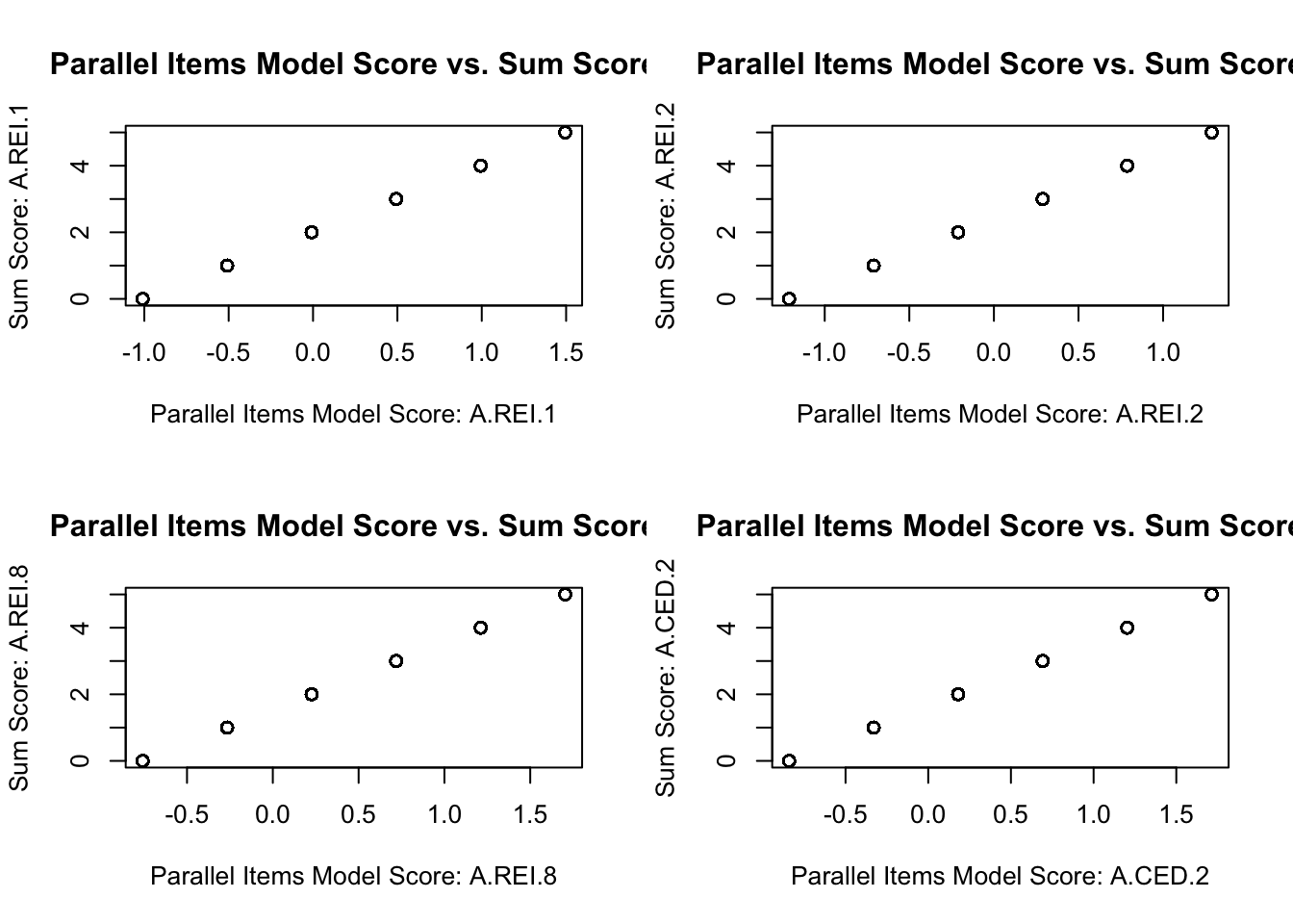
Plotting Sumscores vs. Latent Variable Scores
# create latent variable estimates = lavPredict (parallelItemsModel)# plotting model scores with sumscores par (mfrow = c (2 ,2 ))for (standard in 1 : ncol (reducedQ)){plot (x = parallelItemsScores[, standard], y = sumScores[, standard], main = "Parallel Items Model Score vs. Sum Score" , xlab = paste0 ("Parallel Items Model Score: " , colnames (reducedQ)[standard]), ylab = paste0 ("Sum Score: " , colnames (reducedQ)[standard])
A Better Measurement Model Implied by Subscores
Contrast the unidimensional model with that assumed by the subscores: the multidimensional model
Standards measured (and measurement model):
A.REI.1 (\(\theta_{p1}\) )
\[P(Y_{pi} = 1 | \theta_{p1}) =
\frac{\exp \left(a_i \left( \theta_{p1} - b_i \right) \right)}{1 + \exp \left(a_i \left( \theta_{p1} - b_i \right) \right)} \]
A.REI.2 (\(\theta_{p2}\) )
\[P(Y_{pi} = 1 | \theta_{p2}) = \frac{\exp \left(a_i \left( \theta_{p2} - b_i \right) \right)}{1 + \exp \left(a_i \left( \theta_{p2} - b_i \right) \right)} \]
A.REI.8 (\(\theta_{p3}\) )
\[P(Y_{pi} = 1 | \theta_{p3}) = \frac{\exp \left(a_i \left( \theta_{p3} - b_i \right) \right)}{1 + \exp \left(a_i \left( \theta_{p3} - b_i \right) \right)} \]
A.CED.2 (\(\theta_{p4}\) )
\[P(Y_{pi} = 1 | \theta_{p4}) = \frac{\exp \left(a_i \left( \theta_{p4} - b_i \right) \right)}{1 + \exp \left(a_i \left( \theta_{p4} - b_i \right) \right)} \]
Structural Model Implied by Subscores
\[
\begin{bmatrix}
\theta_{p1} \\
\theta_{p2} \\
\theta_{p3} \\
\theta_{p4} \\
\end{bmatrix}
\sim N \left(\boldsymbol{0}, \boldsymbol{\Sigma}_{M} \right)
\]
Where:
\[
\mathbf{\Sigma}_{M} =
\begin{bmatrix}
1 & \rho_{\theta_1, \theta_2} & \rho_{\theta_1, \theta_3} & \rho_{\theta_1, \theta_4} \\
\rho_{\theta_1, \theta_2} & 1 & \rho_{\theta_2, \theta_3} & \rho_{\theta_2, \theta_4} \\
\rho_{\theta_1, \theta_3} & \rho_{\theta_2, \theta_3} & 1 & \rho_{\theta_3, \theta_4} \\
\rho_{\theta_1, \theta_4} & \rho_{\theta_2, \theta_4} & \rho_{\theta_3, \theta_4} & 1 \\
\end{bmatrix}
\]
Here, \(\mathbf{\Sigma}_{M}\) is a correlation matrix implying identification via standardized factors
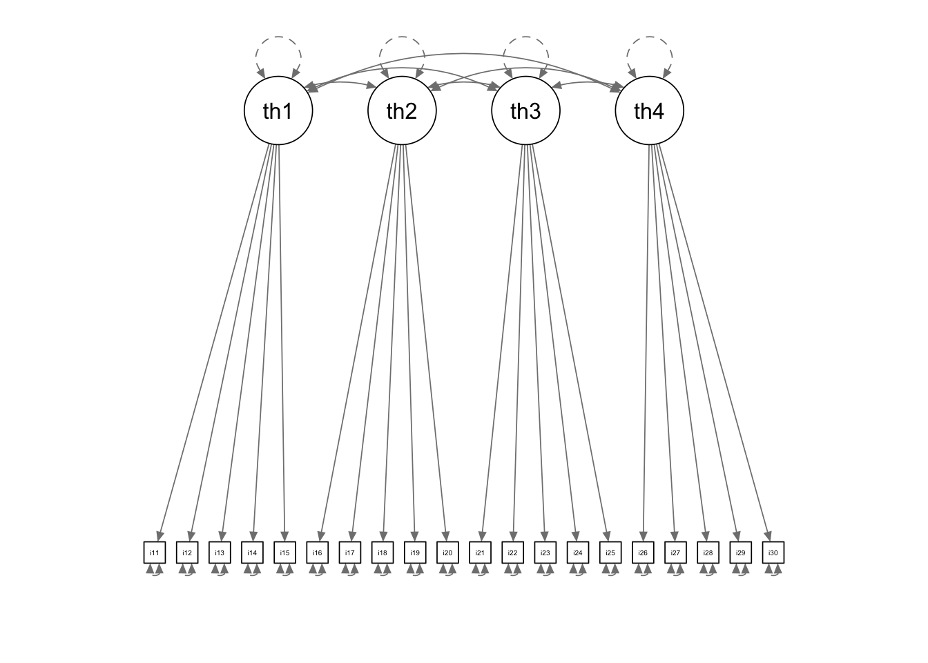
= " theta1 =~ item11 + item12 + item13 + item14 + item15 theta2 =~ item16 + item17 + item18 + item19 + item20 theta3 =~ item21 + item22 + item23 + item24 + item25 theta4 =~ item26 + item27 + item28 + item29 + item30 " = cfa (model = multidimensionalModel_syntax, data = responseMatrix, estimator = "WLSMV" , ordered = paste0 ("item" , 11 : 30 ), std.lv = TRUE , parameterization = "theta" summary (multidimensionalModel, fit.measures = TRUE , standardized = TRUE )
lavaan 0.6.16 ended normally after 26 iterations
Estimator DWLS
Optimization method NLMINB
Number of model parameters 46
Used Total
Number of observations 1099 2541
Model Test User Model:
Standard Scaled
Test Statistic 233.931 298.881
Degrees of freedom 164 164
P-value (Chi-square) 0.000 0.000
Scaling correction factor 0.832
Shift parameter 17.797
simple second-order correction
Model Test Baseline Model:
Test statistic 5341.853 3322.839
Degrees of freedom 190 190
P-value 0.000 0.000
Scaling correction factor 1.644
User Model versus Baseline Model:
Comparative Fit Index (CFI) 0.986 0.957
Tucker-Lewis Index (TLI) 0.984 0.950
Robust Comparative Fit Index (CFI) 0.916
Robust Tucker-Lewis Index (TLI) 0.903
Root Mean Square Error of Approximation:
RMSEA 0.020 0.027
90 Percent confidence interval - lower 0.014 0.022
90 Percent confidence interval - upper 0.025 0.032
P-value H_0: RMSEA <= 0.050 1.000 1.000
P-value H_0: RMSEA >= 0.080 0.000 0.000
Robust RMSEA 0.048
90 Percent confidence interval - lower 0.038
90 Percent confidence interval - upper 0.057
P-value H_0: Robust RMSEA <= 0.050 0.642
P-value H_0: Robust RMSEA >= 0.080 0.000
Standardized Root Mean Square Residual:
SRMR 0.051 0.051
Parameter Estimates:
Standard errors Robust.sem
Information Expected
Information saturated (h1) model Unstructured
Latent Variables:
Estimate Std.Err z-value P(>|z|) Std.lv Std.all
theta1 =~
item11 1.060 0.109 9.769 0.000 1.060 0.727
item12 0.307 0.057 5.362 0.000 0.307 0.294
item13 0.914 0.083 10.988 0.000 0.914 0.675
item14 0.678 0.065 10.470 0.000 0.678 0.561
item15 0.531 0.056 9.410 0.000 0.531 0.469
theta2 =~
item16 0.808 0.067 12.124 0.000 0.808 0.629
item17 0.809 0.069 11.760 0.000 0.809 0.629
item18 1.005 0.086 11.670 0.000 1.005 0.709
item19 1.072 0.090 11.864 0.000 1.072 0.731
item20 0.919 0.098 9.397 0.000 0.919 0.677
theta3 =~
item21 0.227 0.058 3.920 0.000 0.227 0.221
item22 0.419 0.078 5.408 0.000 0.419 0.387
item23 0.679 0.093 7.333 0.000 0.679 0.562
item24 0.593 0.079 7.537 0.000 0.593 0.510
item25 0.680 0.088 7.758 0.000 0.680 0.562
theta4 =~
item26 0.764 0.094 8.152 0.000 0.764 0.607
item27 0.565 0.062 9.161 0.000 0.565 0.492
item28 0.857 0.089 9.609 0.000 0.857 0.651
item29 0.325 0.070 4.665 0.000 0.325 0.309
item30 0.498 0.067 7.434 0.000 0.498 0.446
Covariances:
Estimate Std.Err z-value P(>|z|) Std.lv Std.all
theta1 ~~
theta2 0.754 0.036 20.945 0.000 0.754 0.754
theta3 0.522 0.056 9.336 0.000 0.522 0.522
theta4 0.765 0.044 17.284 0.000 0.765 0.765
theta2 ~~
theta3 0.624 0.047 13.315 0.000 0.624 0.624
theta4 0.583 0.045 12.964 0.000 0.583 0.583
theta3 ~~
theta4 0.542 0.066 8.179 0.000 0.542 0.542
Intercepts:
Estimate Std.Err z-value P(>|z|) Std.lv Std.all
.item11 0.000 0.000 0.000
.item12 0.000 0.000 0.000
.item13 0.000 0.000 0.000
.item14 0.000 0.000 0.000
.item15 0.000 0.000 0.000
.item16 0.000 0.000 0.000
.item17 0.000 0.000 0.000
.item18 0.000 0.000 0.000
.item19 0.000 0.000 0.000
.item20 0.000 0.000 0.000
.item21 0.000 0.000 0.000
.item22 0.000 0.000 0.000
.item23 0.000 0.000 0.000
.item24 0.000 0.000 0.000
.item25 0.000 0.000 0.000
.item26 0.000 0.000 0.000
.item27 0.000 0.000 0.000
.item28 0.000 0.000 0.000
.item29 0.000 0.000 0.000
.item30 0.000 0.000 0.000
theta1 0.000 0.000 0.000
theta2 0.000 0.000 0.000
theta3 0.000 0.000 0.000
theta4 0.000 0.000 0.000
Thresholds:
Estimate Std.Err z-value P(>|z|) Std.lv Std.all
item11|t1 0.507 0.065 7.814 0.000 0.507 0.348
item12|t1 0.649 0.044 14.888 0.000 0.649 0.620
item13|t1 0.138 0.052 2.639 0.008 0.138 0.102
item14|t1 0.137 0.046 2.956 0.003 0.137 0.113
item15|t1 0.084 0.043 1.954 0.051 0.084 0.074
item16|t1 -0.148 0.049 -3.060 0.002 -0.148 -0.115
item17|t1 -0.040 0.049 -0.816 0.415 -0.040 -0.031
item18|t1 -0.047 0.053 -0.877 0.381 -0.047 -0.033
item19|t1 -0.122 0.055 -2.215 0.027 -0.122 -0.083
item20|t1 0.641 0.063 10.109 0.000 0.641 0.472
item21|t1 0.268 0.040 6.797 0.000 0.268 0.262
item22|t1 0.853 0.052 16.444 0.000 0.853 0.787
item23|t1 0.690 0.059 11.726 0.000 0.690 0.571
item24|t1 0.558 0.051 10.915 0.000 0.558 0.480
item25|t1 0.537 0.054 9.898 0.000 0.537 0.444
item26|t1 0.676 0.061 11.023 0.000 0.676 0.537
item27|t1 0.180 0.044 4.071 0.000 0.180 0.157
item28|t1 0.389 0.056 7.001 0.000 0.389 0.295
item29|t1 0.795 0.047 16.808 0.000 0.795 0.756
item30|t1 0.573 0.047 12.089 0.000 0.573 0.513
Variances:
Estimate Std.Err z-value P(>|z|) Std.lv Std.all
.item11 1.000 1.000 0.471
.item12 1.000 1.000 0.914
.item13 1.000 1.000 0.545
.item14 1.000 1.000 0.685
.item15 1.000 1.000 0.780
.item16 1.000 1.000 0.605
.item17 1.000 1.000 0.605
.item18 1.000 1.000 0.497
.item19 1.000 1.000 0.465
.item20 1.000 1.000 0.542
.item21 1.000 1.000 0.951
.item22 1.000 1.000 0.851
.item23 1.000 1.000 0.685
.item24 1.000 1.000 0.740
.item25 1.000 1.000 0.684
.item26 1.000 1.000 0.631
.item27 1.000 1.000 0.758
.item28 1.000 1.000 0.576
.item29 1.000 1.000 0.904
.item30 1.000 1.000 0.801
theta1 1.000 1.000 1.000
theta2 1.000 1.000 1.000
theta3 1.000 1.000 1.000
theta4 1.000 1.000 1.000
Scales y*:
Estimate Std.Err z-value P(>|z|) Std.lv Std.all
item11 0.686 0.686 1.000
item12 0.956 0.956 1.000
item13 0.738 0.738 1.000
item14 0.828 0.828 1.000
item15 0.883 0.883 1.000
item16 0.778 0.778 1.000
item17 0.778 0.778 1.000
item18 0.705 0.705 1.000
item19 0.682 0.682 1.000
item20 0.736 0.736 1.000
item21 0.975 0.975 1.000
item22 0.922 0.922 1.000
item23 0.827 0.827 1.000
item24 0.860 0.860 1.000
item25 0.827 0.827 1.000
item26 0.795 0.795 1.000
item27 0.871 0.871 1.000
item28 0.759 0.759 1.000
item29 0.951 0.951 1.000
item30 0.895 0.895 1.000
Multidimensional Model Path Diagram
:: semPaths (multidimensionalModel, sizeMan = 2.5 , style = "mx" , intercepts = FALSE , thresholds = FALSE )
Model Score Comparisons
= lavPredict (multidimensionalModel)= data.frame (cbind (unidimensionalScores, multidimensionalScores))names (allScores) = c ("uTheta" , paste0 ("mTheta" , 1 : 4 ))plot (allScores, main = "Unidimensional Score vs. Multidimensional Scores" )
           uTheta   mTheta1   mTheta2   mTheta3   mTheta4
uTheta  1.0000000 0.9763872 0.9734620 0.8953982 0.9324452
mTheta1 0.9763872 1.0000000 0.9249558 0.8119392 0.9400688
mTheta2 0.9734620 0.9249558 1.0000000 0.8657125 0.8361691
mTheta3 0.8953982 0.8119392 0.8657125 1.0000000 0.8101180
mTheta4 0.9324452 0.9400688 0.8361691 0.8101180 1.0000000
Model Fit Comparison
Which model fits the data better? Chi-square difference test:
Note: Comparison is only unidimensional IRT model vs. Multidimensional IRT model
Sumscore-based MCFA model not comparable as likelihood is on different scale
Observed variables Bernoulli distributed in IRT
Observed variables normally distributed in CFA
anova (unidimensionalModel, multidimensionalModel)
Scaled Chi-Squared Difference Test (method = "satorra.2000")

lavaan NOTE:
    The "Chisq" column contains standard test statistics, not the
    robust test that should be reported per model. A robust difference
    test is a function of two standard (not robust) statistics.

                       Df AIC BIC  Chisq Chisq diff Df diff Pr(>Chisq)
multidimensionalModel 164         233.93
unidimensionalModel   170         419.00      146.5       6  < 2.2e-16 ***
---
Signif. codes:  0 '***' 0.001 '**' 0.01 '*' 0.05 '.' 0.1 ' ' 1
The MIRT model fits better than the unidimensional model
So, if reporting both types of scores, discrepancies can arise
Differing models may have competing information
Which score is more accurate?
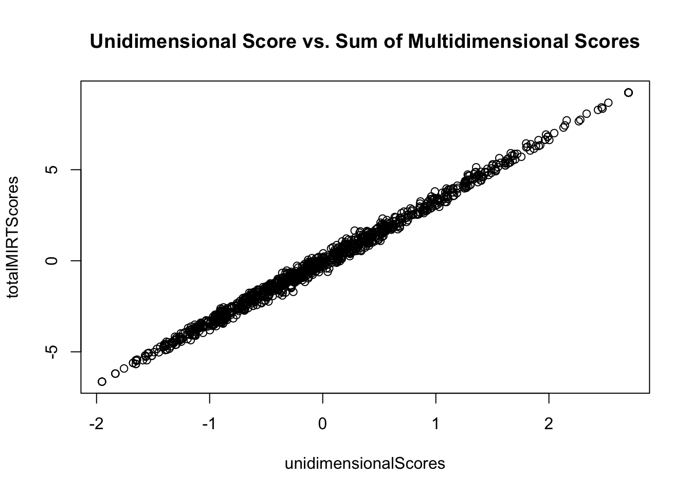
Option 2: Summed Multidimensional Model Scores
Another option for reporting subscores and an overall score is to:
Estimate subscores from the MIRT model
Create the total score with the sum of each of the latent variable estimates from the MIRT model:
= rowSums (multidimensionalScores)plot (x = unidimensionalScores, y = totalMIRTScores, main = "Unidimensional Score vs. Sum of Multidimensional Scores" )cor (x = unidimensionalScores, y = totalMIRTScores)
Evaluating Option 2
Option 2 is closer to what is needed in that it uses MIRT to form a total score
But, what is the model that Option 2 implies?
\[
\begin{array}{c}
\theta_{p1} = \mu_1 + \lambda F + e_{p1}; e \sim N(0, \psi^2) \\
\theta_{p2} = \mu_2 + \lambda F + e_{p2}; e \sim N(0, \psi^2) \\
\theta_{p3} = \mu_3 + \lambda F + e_{p3}; e \sim N(0, \psi^2) \\
\theta_{p4} = \mu_4 + \lambda F + e_{p4}; e \sim N(0, \psi^2) \\
\end{array}
\]
Where \(F \sim N(0, 1)\)
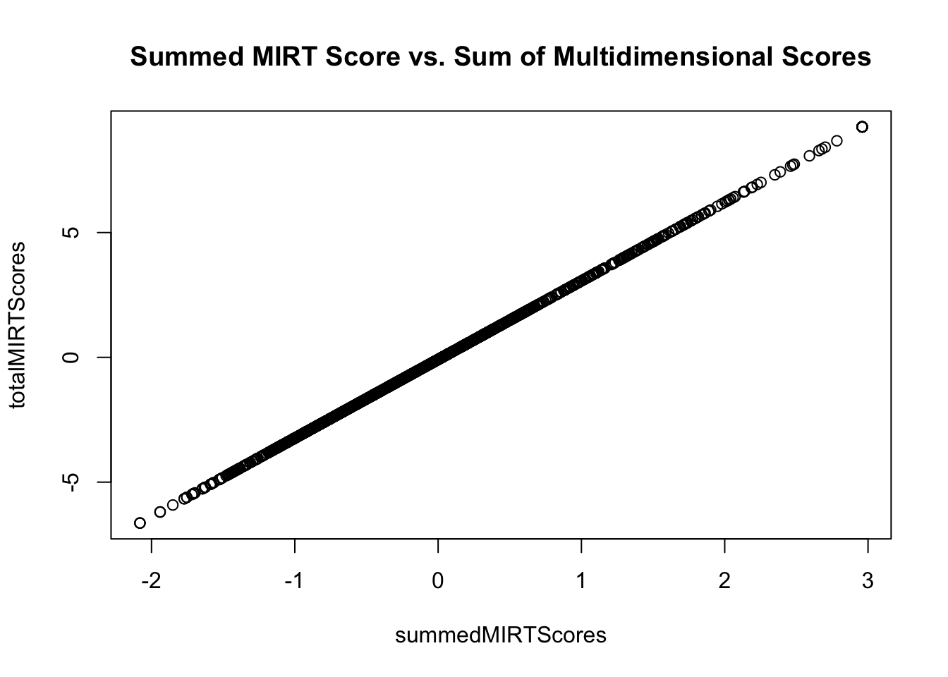
Testing if Summed MIRT Score Model Fits Data
= " # constrain all loadings to be equal total =~ L1*theta1 + L1*theta2 + L1*theta3 + L1*theta4 # set the unique variances to be equal theta1 ~~ U1*theta1; theta2 ~~ U1*theta2; theta3 ~~ U1*theta3; theta4 ~~ U1*theta4; " = cfa (model = summedMIRT_syntax, data = multidimensionalScores, estimator = "MLR" ,std.lv = TRUE , summary (summedMIRTModel, fit.measures = TRUE , standardized = TRUE )
lavaan 0.6.15 ended normally after 10 iterations

  Estimator                                         ML
  Optimization method                           NLMINB
  Number of model parameters                         8
  Number of equality constraints                     6

  Number of observations                          1099

Model Test User Model:
                                              Standard      Scaled
  Test Statistic                              1240.195    1493.422
  Degrees of freedom                                 8           8
  P-value (Chi-square)                           0.000       0.000
  Scaling correction factor                                  0.830
    Yuan-Bentler correction (Mplus variant)

Model Test Baseline Model:

  Test statistic                              6334.409    8515.633
  Degrees of freedom                                 6           6
  P-value                                        0.000       0.000
  Scaling correction factor                                  0.744

User Model versus Baseline Model:

  Comparative Fit Index (CFI)                    0.805       0.825
  Tucker-Lewis Index (TLI)                       0.854       0.869

  Robust Comparative Fit Index (CFI)                         0.805
  Robust Tucker-Lewis Index (TLI)                            0.854

Loglikelihood and Information Criteria:

  Loglikelihood user model (H0)              -2772.002   -2772.002
  Scaling correction factor                                  0.303
      for the MLR correction
  Loglikelihood unrestricted model (H1)      -2151.905   -2151.905
  Scaling correction factor                                  0.907
      for the MLR correction

  Akaike (AIC)                                5548.005    5548.005
  Bayesian (BIC)                              5558.009    5558.009
  Sample-size adjusted Bayesian (SABIC)       5551.657    5551.657

Root Mean Square Error of Approximation:

  RMSEA                                          0.374       0.411
  90 Percent confidence interval - lower         0.357       0.392
  90 Percent confidence interval - upper         0.392       0.430
  P-value H_0: RMSEA <= 0.050                    0.000       0.000
  P-value H_0: RMSEA >= 0.080                    1.000       1.000

  Robust RMSEA                                               0.375
  90 Percent confidence interval - lower                     0.359
  90 Percent confidence interval - upper                     0.391
  P-value H_0: Robust RMSEA <= 0.050                         0.000
  P-value H_0: Robust RMSEA >= 0.080                         1.000

Standardized Root Mean Square Residual:

  SRMR                                           0.128       0.128

Parameter Estimates:

  Standard errors                             Sandwich
  Information bread                           Observed
  Observed information based on                Hessian

Latent Variables:
                   Estimate  Std.Err  z-value  P(>|z|)   Std.lv  Std.all
  total =~
    theta1    (L1)    0.757    0.019   40.075    0.000    0.757    0.929
    theta2    (L1)    0.757    0.019   40.075    0.000    0.757    0.929
    theta3    (L1)    0.757    0.019   40.075    0.000    0.757    0.929
    theta4    (L1)    0.757    0.019   40.075    0.000    0.757    0.929

Variances:
                   Estimate  Std.Err  z-value  P(>|z|)   Std.lv  Std.all
   .theta1    (U1)    0.091    0.002   37.596    0.000    0.091    0.138
   .theta2    (U1)    0.091    0.002   37.596    0.000    0.091    0.138
   .theta3    (U1)    0.091    0.002   37.596    0.000    0.091    0.138
   .theta4    (U1)    0.091    0.002   37.596    0.000    0.091    0.138
    total             1.000                               1.000    1.000
Demonstrating Equivalence (Scalar) with Summed MIRT Scores
= lavPredict (summedMIRTModel)plot (x = summedMIRTScores, y = totalMIRTScores, main = "Summed MIRT Score vs. Sum of Multidimensional Scores" )
Option #3: Bifactor Model
A bifactor model is a multidimensional model where:
Each item loads on a general factor and a specific factor
The general factor is uncorrelated with the specific factors
The specific factors can be uncorrelated with each other (as a method factor) or correlated with each other (as a multidimensional model)
Bifactor Model Notation
The bifactor model is:
Subscore 1:
\[
\begin{array}{c}
\text{logit}\left( P\left( Y_{p1} = 1 \mid \theta_{p1}, g_p \right) \right) = \mu_1 + \lambda_{11} \theta_{p1} + \lambda_{1g} g_p \\
\text{logit}\left( P\left( Y_{p2} = 1 \mid \theta_{p2}, g_p \right) \right) = \mu_2 + \lambda_{21} \theta_{p1} + \lambda_{2g} g_p \\
\vdots \\
\text{logit}\left( P\left( Y_{p5} = 1 \mid \theta_{p5}, g_p \right) \right) = \mu_5 + \lambda_{51} \theta_{p1} + \lambda_{5g} g_p \\
\end{array}
\]
Subscore 2:
\[
\begin{array}{c}
\text{logit}\left( P\left( Y_{p6} = 1 \mid \theta_{p6}, g_p \right) \right) = \mu_6 + \lambda_{61} \theta_{p2} + \lambda_{6g} g_p \\
\text{logit}\left( P\left( Y_{p7} = 1 \mid \theta_{p7}, g_p \right) \right) = \mu_7 + \lambda_{71} \theta_{p2} + \lambda_{7g} g_p \\
\vdots \\
\text{logit}\left( P\left( Y_{p10} = 1 \mid \theta_{p10}, g_p \right) \right) = \mu_{10} + \lambda_{101} \theta_{p2} + \lambda_{10g} g_p \\
\end{array}
\]
Bifactor Model in lavaan
= " g =~ item11 + item12 + item13 + item14 + item15 + item16 + item17 + item18 + item19 + item20 + item21 + item22 + item23 + item24 + item25 + item26 + item27 + item28 + item29 + item30 theta1 =~ item11 + item12 + item13 + item14 + item15 theta2 =~ item16 + item17 + item18 + item19 + item20 theta3 =~ item21 + item22 + item23 + item24 + item25 theta4 =~ item26 + item27 + item28 + item29 + item30 g ~~ 0*theta1 g ~~ 0*theta2 g ~~ 0*theta3 g ~~ 0*theta4 " = cfa (model = bifactorModel_syntax, data = responseMatrix, estimator = "WLSMV" , ordered = paste0 ("item" , 11 : 30 ), std.lv = TRUE , parameterization = "theta" summary (bifactorModel, fit.measures = TRUE , standardized = TRUE )
lavaan 0.6.15 ended normally after 85 iterations
Estimator DWLS
Optimization method NLMINB
Number of model parameters 66
Used Total
Number of observations 1099 2541
Model Test User Model:
Standard Scaled
Test Statistic 122.416 169.422
Degrees of freedom 144 144
P-value (Chi-square) 0.904 0.073
Scaling correction factor 0.787
Shift parameter 13.922
simple second-order correction
Model Test Baseline Model:
Test statistic 5341.853 3322.839
Degrees of freedom 190 190
P-value 0.000 0.000
Scaling correction factor 1.644
User Model versus Baseline Model:
Comparative Fit Index (CFI) 1.000 0.992
Tucker-Lewis Index (TLI) 1.006 0.989
Robust Comparative Fit Index (CFI) 0.977
Robust Tucker-Lewis Index (TLI) 0.969
Root Mean Square Error of Approximation:
RMSEA 0.000 0.013
90 Percent confidence interval - lower 0.000 0.000
90 Percent confidence interval - upper 0.006 0.020
P-value H_0: RMSEA <= 0.050 1.000 1.000
P-value H_0: RMSEA >= 0.080 0.000 0.000
Robust RMSEA 0.027
90 Percent confidence interval - lower 0.005
90 Percent confidence interval - upper 0.040
P-value H_0: Robust RMSEA <= 0.050 0.999
P-value H_0: Robust RMSEA >= 0.080 0.000
Standardized Root Mean Square Residual:
SRMR 0.037 0.037
Parameter Estimates:
Standard errors Robust.sem
Information Expected
Information saturated (h1) model Unstructured
Latent Variables:
Estimate Std.Err z-value P(>|z|) Std.lv Std.all
g =~
item11 0.746 0.098 7.627 0.000 0.746 0.505
item12 0.364 0.071 5.161 0.000 0.364 0.342
item13 0.615 0.083 7.454 0.000 0.615 0.439
item14 0.495 0.067 7.333 0.000 0.495 0.410
item15 0.416 0.060 6.956 0.000 0.416 0.369
item16 0.291 0.082 3.557 0.000 0.291 0.201
item17 0.396 0.068 5.803 0.000 0.396 0.304
item18 0.524 0.078 6.715 0.000 0.524 0.369
item19 0.551 0.083 6.664 0.000 0.551 0.375
item20 0.683 0.083 8.276 0.000 0.683 0.519
item21 0.213 0.056 3.835 0.000 0.213 0.208
item22 0.409 0.077 5.279 0.000 0.409 0.378
item23 0.470 0.077 6.098 0.000 0.470 0.396
item24 0.351 0.101 3.482 0.000 0.351 0.242
item25 0.457 0.075 6.137 0.000 0.457 0.382
item26 0.755 0.094 8.064 0.000 0.755 0.597
item27 0.396 0.074 5.346 0.000 0.396 0.327
item28 0.727 0.171 4.245 0.000 0.727 0.439
item29 0.402 0.079 5.056 0.000 0.402 0.372
item30 0.527 0.074 7.148 0.000 0.527 0.466
theta1 =~
item11 0.792 0.133 5.943 0.000 0.792 0.536
item12 0.020 0.078 0.260 0.795 0.020 0.019
item13 0.762 0.119 6.389 0.000 0.762 0.544
item14 0.460 0.088 5.216 0.000 0.460 0.381
item15 0.315 0.078 4.063 0.000 0.315 0.279
theta2 =~
item16 1.003 0.126 7.941 0.000 1.003 0.694
item17 0.736 0.087 8.432 0.000 0.736 0.565
item18 0.860 0.101 8.533 0.000 0.860 0.606
item19 0.926 0.108 8.558 0.000 0.926 0.630
item20 0.517 0.087 5.965 0.000 0.517 0.392
theta3 =~
item21 0.070 0.065 1.069 0.285 0.070 0.068
item22 0.039 0.077 0.498 0.618 0.039 0.036
item23 0.435 0.095 4.590 0.000 0.435 0.367
item24 0.991 0.250 3.973 0.000 0.991 0.683
item25 0.477 0.097 4.917 0.000 0.477 0.398
theta4 =~
item26 0.171 0.100 1.709 0.087 0.171 0.135
item27 0.557 0.130 4.283 0.000 0.557 0.460
item28 1.100 0.374 2.939 0.003 1.100 0.665
item29 -0.072 0.090 -0.792 0.428 -0.072 -0.066
item30 0.040 0.093 0.429 0.668 0.040 0.035
Covariances:
Estimate Std.Err z-value P(>|z|) Std.lv Std.all
g ~~
theta1 0.000 0.000 0.000
theta2 0.000 0.000 0.000
theta3 0.000 0.000 0.000
theta4 0.000 0.000 0.000
theta1 ~~
theta2 0.619 0.065 9.571 0.000 0.619 0.619
theta3 0.018 0.114 0.161 0.872 0.018 0.018
theta4 0.430 0.111 3.880 0.000 0.430 0.430
theta2 ~~
theta3 0.419 0.074 5.702 0.000 0.419 0.419
theta4 0.275 0.090 3.072 0.002 0.275 0.275
theta3 ~~
theta4 -0.068 0.114 -0.599 0.549 -0.068 -0.068
Intercepts:
Estimate Std.Err z-value P(>|z|) Std.lv Std.all
.item11 0.000 0.000 0.000
.item12 0.000 0.000 0.000
.item13 0.000 0.000 0.000
.item14 0.000 0.000 0.000
.item15 0.000 0.000 0.000
.item16 0.000 0.000 0.000
.item17 0.000 0.000 0.000
.item18 0.000 0.000 0.000
.item19 0.000 0.000 0.000
.item20 0.000 0.000 0.000
.item21 0.000 0.000 0.000
.item22 0.000 0.000 0.000
.item23 0.000 0.000 0.000
.item24 0.000 0.000 0.000
.item25 0.000 0.000 0.000
.item26 0.000 0.000 0.000
.item27 0.000 0.000 0.000
.item28 0.000 0.000 0.000
.item29 0.000 0.000 0.000
.item30 0.000 0.000 0.000
g 0.000 0.000 0.000
theta1 0.000 0.000 0.000
theta2 0.000 0.000 0.000
theta3 0.000 0.000 0.000
theta4 0.000 0.000 0.000
Thresholds:
Estimate Std.Err z-value P(>|z|) Std.lv Std.all
item11|t1 0.514 0.067 7.644 0.000 0.514 0.348
item12|t1 0.660 0.046 14.349 0.000 0.660 0.620
item13|t1 0.142 0.054 2.631 0.009 0.142 0.102
item14|t1 0.137 0.046 2.957 0.003 0.137 0.113
item15|t1 0.084 0.043 1.954 0.051 0.084 0.074
item16|t1 -0.167 0.055 -3.029 0.002 -0.167 -0.115
item17|t1 -0.040 0.049 -0.815 0.415 -0.040 -0.031
item18|t1 -0.047 0.054 -0.876 0.381 -0.047 -0.033
item19|t1 -0.123 0.056 -2.207 0.027 -0.123 -0.083
item20|t1 0.621 0.059 10.475 0.000 0.621 0.472
item21|t1 0.268 0.039 6.804 0.000 0.268 0.262
item22|t1 0.851 0.052 16.506 0.000 0.851 0.787
item23|t1 0.679 0.056 12.119 0.000 0.679 0.571
item24|t1 0.696 0.108 6.468 0.000 0.696 0.480
item25|t1 0.532 0.053 10.035 0.000 0.532 0.444
item26|t1 0.679 0.062 11.017 0.000 0.679 0.537
item27|t1 0.190 0.047 4.008 0.000 0.190 0.157
item28|t1 0.488 0.113 4.334 0.000 0.488 0.295
item29|t1 0.817 0.052 15.670 0.000 0.817 0.756
item30|t1 0.580 0.049 11.860 0.000 0.580 0.513
Variances:
Estimate Std.Err z-value P(>|z|) Std.lv Std.all
.item11 1.000 1.000 0.458
.item12 1.000 1.000 0.882
.item13 1.000 1.000 0.511
.item14 1.000 1.000 0.687
.item15 1.000 1.000 0.786
.item16 1.000 1.000 0.478
.item17 1.000 1.000 0.589
.item18 1.000 1.000 0.497
.item19 1.000 1.000 0.463
.item20 1.000 1.000 0.577
.item21 1.000 1.000 0.952
.item22 1.000 1.000 0.856
.item23 1.000 1.000 0.709
.item24 1.000 1.000 0.475
.item25 1.000 1.000 0.696
.item26 1.000 1.000 0.626
.item27 1.000 1.000 0.682
.item28 1.000 1.000 0.365
.item29 1.000 1.000 0.857
.item30 1.000 1.000 0.782
g 1.000 1.000 1.000
theta1 1.000 1.000 1.000
theta2 1.000 1.000 1.000
theta3 1.000 1.000 1.000
theta4 1.000 1.000 1.000
Scales y*:
Estimate Std.Err z-value P(>|z|) Std.lv Std.all
item11 0.677 0.677 1.000
item12 0.939 0.939 1.000
item13 0.715 0.715 1.000
item14 0.829 0.829 1.000
item15 0.887 0.887 1.000
item16 0.692 0.692 1.000
item17 0.767 0.767 1.000
item18 0.705 0.705 1.000
item19 0.680 0.680 1.000
item20 0.759 0.759 1.000
item21 0.976 0.976 1.000
item22 0.925 0.925 1.000
item23 0.842 0.842 1.000
item24 0.689 0.689 1.000
item25 0.834 0.834 1.000
item26 0.791 0.791 1.000
item27 0.826 0.826 1.000
item28 0.604 0.604 1.000
item29 0.926 0.926 1.000
item30 0.884 0.884 1.000
Bifactor Model Path Diagram
:: semPaths (bifactorModel, sizeMan = 2.5 , style = "mx" , intercepts = FALSE , thresholds = FALSE )
Note: as rendered when this lecture was constructed, the plot has correlations between \(g\) and the \(\theta\) , which are not present in the model
Bifactor Model Score Comparisons: Unidimensional IRT model \(\theta\) vs. Bifactor IRT model \(g\)
= lavPredict (bifactorModel)plot (x = unidimensionalScores, y = bifactorScores[, "g" ], main = "Unidimensional Score vs. Bifactor Score" )
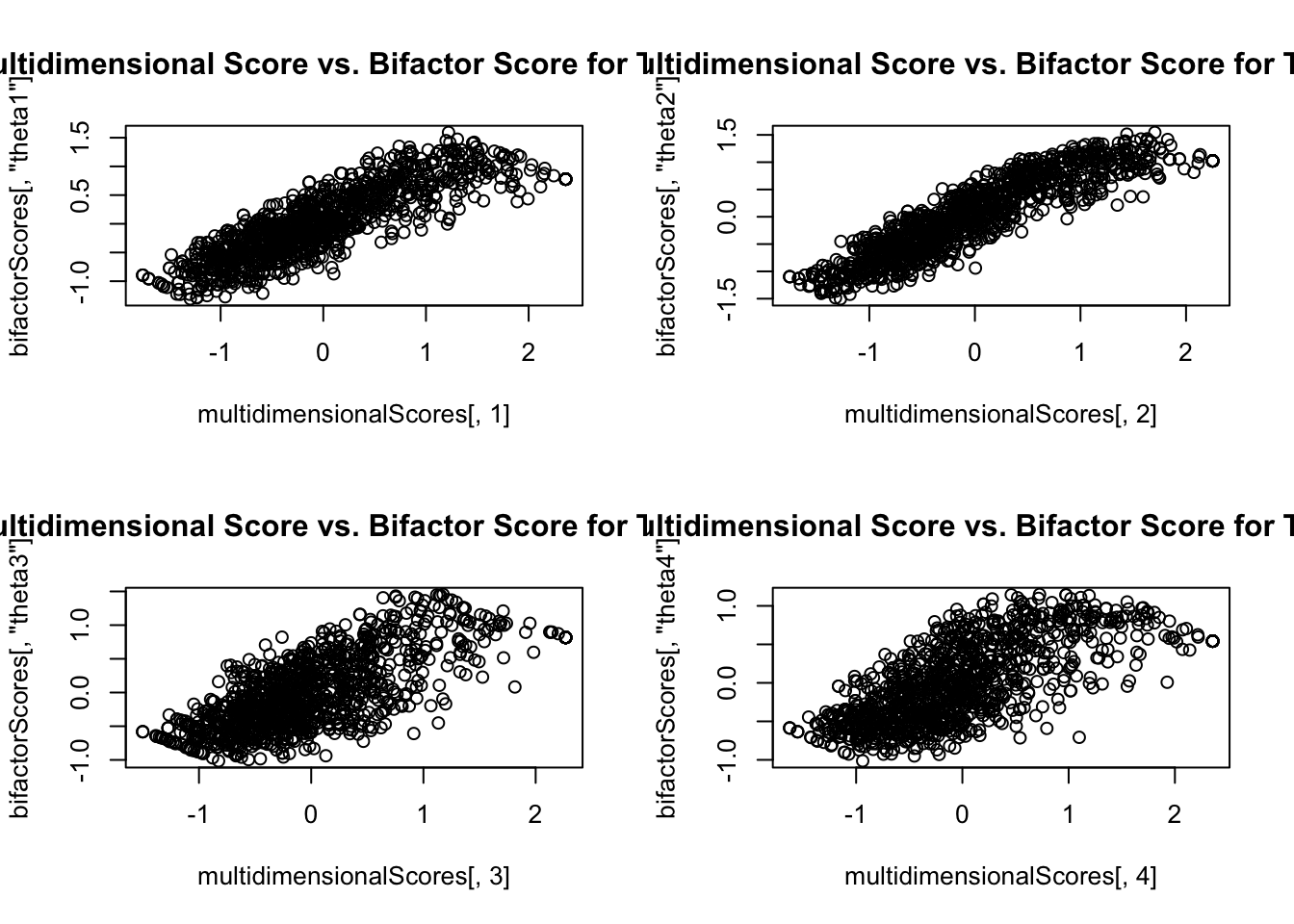
Bifactor Model Score Comparisons: Standards
par (mfrow = c (2 ,2 ))plot (x = multidimensionalScores[, 1 ], y = bifactorScores[, "theta1" ],main = "Multidimensional Score vs. Bifactor Score for Theta 1" )plot (x = multidimensionalScores[, 2 ], y = bifactorScores[, "theta2" ],main = "Multidimensional Score vs. Bifactor Score for Theta 1" )plot (x = multidimensionalScores[, 3 ], y = bifactorScores[, "theta3" ],main = "Multidimensional Score vs. Bifactor Score for Theta 1" )plot (x = multidimensionalScores[, 4 ], y = bifactorScores[, "theta4" ],main = "Multidimensional Score vs. Bifactor Score for Theta 1" )
From Score Plot: Scores are Not Same
The bifactor model scores are not the same as the multidimensional model scores
The general factor is not the same as total score in the unidimensional model
Rather, it is the score of the domain that does not include the subdomains
Put another way: It is everything left over in algebra after controlling for a person’s ability in the algebra standards
Sometimes considered a residual
Model Fit Comparison
But…the bifactor model nearly always fits better than a similar multidimensional model
anova (unidimensionalModel, multidimensionalModel, bifactorModel)
Scaled Chi-Squared Difference Test (method = "satorra.2000")

lavaan NOTE:
    The "Chisq" column contains standard test statistics, not the
    robust test that should be reported per model. A robust difference
    test is a function of two standard (not robust) statistics.

                       Df AIC BIC  Chisq Chisq diff Df diff Pr(>Chisq)
bifactorModel         144         122.42
multidimensionalModel 164         233.93     110.74      20  1.442e-14 ***
unidimensionalModel   170         419.00     146.50       6  < 2.2e-16 ***
---
Signif. codes:  0 '***' 0.001 '**' 0.01 '*' 0.05 '.' 0.1 ' ' 1
Option #4: Higher Order Model
A higher order model is a multidimensional model where:
Each item loads onto its subdomain factor, identically with the multidimensional model (MIRT)
Each factor then loads onto a general factor
Higher Order Model Notation
Subscore 1:
\[
\begin{array}{c}
\text{logit}\left( P\left( Y_{p1} = 1 \mid \theta_{p1} \right) \right) = \mu_1 + \lambda_{11} \theta_{p1} \\
\text{logit}\left( P\left( Y_{p2} = 1 \mid \theta_{p2} \right) \right) = \mu_2 + \lambda_{21} \theta_{p1} \\
\vdots \\
\text{logit}\left( P\left( Y_{p5} = 1 \mid \theta_{p5} \right) \right) = \mu_5 + \lambda_{51} \theta_{p1} \\
\end{array}
\]
Subscore 2:
\[
\begin{array}{c}
\text{logit}\left( P\left( Y_{p6} = 1 \mid \theta_{p6} \right) \right) = \mu_6 + \lambda_{61} \theta_{p2} \\
\text{logit}\left( P\left( Y_{p7} = 1 \mid \theta_{p7} \right) \right) = \mu_7 + \lambda_{71} \theta_{p2} \\
\vdots \\
\text{logit}\left( P\left( Y_{p10} = 1 \mid \theta_{p10} \right) \right) = \mu_{10} + \lambda_{101} \theta_{p2} \\
\end{array}
\]
Structural Model – a unidimensional CFA model for the subdomains:
\[
\begin{array}{c}
\theta_{p1} = \mu_1 + \lambda_{1} F + e_{p1}; e_{p1} \sim N(0, \psi^2_1) \\
\theta_{p2} = \mu_2 + \lambda_{2} F + e_{p2}; e_{p2} \sim N(0, \psi^2_2) \\
\theta_{p3} = \mu_3 + \lambda_{3} F + e_{p3}; e_{p3} \sim N(0, \psi^2_3) \\
\theta_{p4} = \mu_4 + \lambda_{4} F + e_{p4}; e_{p4} \sim N(0, \psi^2_4) \\
\end{array}
\]
Model-Implied Covariance Matrix of Subdomain Latent Variables
\[
\begin{bmatrix}
\theta_{p1} \\
\theta_{p2} \\
\theta_{p3} \\
\theta_{p4} \\
\end{bmatrix}
\sim N \left(\boldsymbol{0}, \boldsymbol{\Sigma}_{M} \right)
\]
Where:
\[
\mathbf{\Sigma}_{M} = \mathbf{\Lambda} \mathbf{\Phi} \mathbf{\Lambda}^T + \boldsymbol{\Psi}
\]
So, the higher order model is the MIRT model with a more restricted structure on the covariance matrix of the subdomain latent variables
Higher Order Model in lavaan
= " theta1 =~ item11 + item12 + item13 + item14 + item15 theta2 =~ item16 + item17 + item18 + item19 + item20 theta3 =~ item21 + item22 + item23 + item24 + item25 theta4 =~ item26 + item27 + item28 + item29 + item30 algebra =~ theta1 + theta2 + theta3 + theta4 " = cfa (model = higherOrderModel_syntax, data = responseMatrix, estimator = "WLSMV" , ordered = paste0 ("item" , 11 : 30 ), std.lv = TRUE , parameterization = "theta" summary (higherOrderModel, fit.measures = TRUE , standardized = TRUE )
lavaan 0.6.15 ended normally after 47 iterations
Estimator DWLS
Optimization method NLMINB
Number of model parameters 44
Used Total
Number of observations 1099 2541
Model Test User Model:
Standard Scaled
Test Statistic 252.420 317.925
Degrees of freedom 166 166
P-value (Chi-square) 0.000 0.000
Scaling correction factor 0.843
Shift parameter 18.646
simple second-order correction
Model Test Baseline Model:
Test statistic 5341.853 3322.839
Degrees of freedom 190 190
P-value 0.000 0.000
Scaling correction factor 1.644
User Model versus Baseline Model:
Comparative Fit Index (CFI) 0.983 0.952
Tucker-Lewis Index (TLI) 0.981 0.944
Robust Comparative Fit Index (CFI) 0.907
Robust Tucker-Lewis Index (TLI) 0.894
Root Mean Square Error of Approximation:
RMSEA 0.022 0.029
90 Percent confidence interval - lower 0.016 0.024
90 Percent confidence interval - upper 0.027 0.034
P-value H_0: RMSEA <= 0.050 1.000 1.000
P-value H_0: RMSEA >= 0.080 0.000 0.000
Robust RMSEA 0.050
90 Percent confidence interval - lower 0.040
90 Percent confidence interval - upper 0.059
P-value H_0: Robust RMSEA <= 0.050 0.501
P-value H_0: Robust RMSEA >= 0.080 0.000
Standardized Root Mean Square Residual:
SRMR 0.053 0.053
Parameter Estimates:
Standard errors Robust.sem
Information Expected
Information saturated (h1) model Unstructured
Latent Variables:
Estimate Std.Err z-value P(>|z|) Std.lv Std.all
theta1 =~
item11 0.425 0.102 4.153 0.000 1.057 0.726
item12 0.124 0.034 3.692 0.000 0.309 0.295
item13 0.367 0.086 4.282 0.000 0.913 0.674
item14 0.272 0.063 4.315 0.000 0.675 0.560
item15 0.215 0.050 4.287 0.000 0.534 0.471
theta2 =~
item16 0.463 0.054 8.583 0.000 0.808 0.628
item17 0.464 0.055 8.394 0.000 0.809 0.629
item18 0.575 0.070 8.195 0.000 1.003 0.708
item19 0.614 0.074 8.326 0.000 1.071 0.731
item20 0.529 0.072 7.300 0.000 0.922 0.678
theta3 =~
item21 0.168 0.043 3.946 0.000 0.229 0.223
item22 0.312 0.059 5.306 0.000 0.426 0.392
item23 0.498 0.076 6.551 0.000 0.680 0.563
item24 0.424 0.062 6.847 0.000 0.579 0.501
item25 0.499 0.074 6.769 0.000 0.681 0.563
theta4 =~
item26 0.485 0.074 6.591 0.000 0.768 0.609
item27 0.356 0.047 7.504 0.000 0.563 0.491
item28 0.544 0.075 7.231 0.000 0.860 0.652
item29 0.205 0.045 4.533 0.000 0.324 0.308
item30 0.314 0.048 6.545 0.000 0.496 0.444
algebra =~
theta1 2.276 0.539 4.225 0.000 0.916 0.916
theta2 1.429 0.167 8.557 0.000 0.819 0.819
theta3 0.929 0.122 7.601 0.000 0.681 0.681
theta4 1.225 0.159 7.692 0.000 0.775 0.775
Intercepts:
Estimate Std.Err z-value P(>|z|) Std.lv Std.all
.item11 0.000 0.000 0.000
.item12 0.000 0.000 0.000
.item13 0.000 0.000 0.000
.item14 0.000 0.000 0.000
.item15 0.000 0.000 0.000
.item16 0.000 0.000 0.000
.item17 0.000 0.000 0.000
.item18 0.000 0.000 0.000
.item19 0.000 0.000 0.000
.item20 0.000 0.000 0.000
.item21 0.000 0.000 0.000
.item22 0.000 0.000 0.000
.item23 0.000 0.000 0.000
.item24 0.000 0.000 0.000
.item25 0.000 0.000 0.000
.item26 0.000 0.000 0.000
.item27 0.000 0.000 0.000
.item28 0.000 0.000 0.000
.item29 0.000 0.000 0.000
.item30 0.000 0.000 0.000
.theta1 0.000 0.000 0.000
.theta2 0.000 0.000 0.000
.theta3 0.000 0.000 0.000
.theta4 0.000 0.000 0.000
algebra 0.000 0.000 0.000
Thresholds:
Estimate Std.Err z-value P(>|z|) Std.lv Std.all
item11|t1 0.506 0.065 7.821 0.000 0.506 0.348
item12|t1 0.649 0.044 14.879 0.000 0.649 0.620
item13|t1 0.138 0.052 2.639 0.008 0.138 0.102
item14|t1 0.137 0.046 2.956 0.003 0.137 0.113
item15|t1 0.084 0.043 1.953 0.051 0.084 0.074
item16|t1 -0.148 0.049 -3.060 0.002 -0.148 -0.115
item17|t1 -0.040 0.049 -0.816 0.415 -0.040 -0.031
item18|t1 -0.047 0.053 -0.877 0.381 -0.047 -0.033
item19|t1 -0.122 0.055 -2.215 0.027 -0.122 -0.083
item20|t1 0.642 0.064 10.093 0.000 0.642 0.472
item21|t1 0.269 0.040 6.795 0.000 0.269 0.262
item22|t1 0.855 0.052 16.352 0.000 0.855 0.787
item23|t1 0.691 0.059 11.691 0.000 0.691 0.571
item24|t1 0.554 0.051 10.964 0.000 0.554 0.480
item25|t1 0.537 0.054 9.881 0.000 0.537 0.444
item26|t1 0.677 0.062 10.991 0.000 0.677 0.537
item27|t1 0.180 0.044 4.071 0.000 0.180 0.157
item28|t1 0.389 0.056 6.990 0.000 0.389 0.295
item29|t1 0.795 0.047 16.813 0.000 0.795 0.756
item30|t1 0.573 0.047 12.091 0.000 0.573 0.513
Variances:
Estimate Std.Err z-value P(>|z|) Std.lv Std.all
.item11 1.000 1.000 0.472
.item12 1.000 1.000 0.913
.item13 1.000 1.000 0.545
.item14 1.000 1.000 0.687
.item15 1.000 1.000 0.778
.item16 1.000 1.000 0.605
.item17 1.000 1.000 0.604
.item18 1.000 1.000 0.499
.item19 1.000 1.000 0.466
.item20 1.000 1.000 0.540
.item21 1.000 1.000 0.950
.item22 1.000 1.000 0.847
.item23 1.000 1.000 0.684
.item24 1.000 1.000 0.749
.item25 1.000 1.000 0.683
.item26 1.000 1.000 0.629
.item27 1.000 1.000 0.759
.item28 1.000 1.000 0.575
.item29 1.000 1.000 0.905
.item30 1.000 1.000 0.803
.theta1 1.000 0.162 0.162
.theta2 1.000 0.329 0.329
.theta3 1.000 0.537 0.537
.theta4 1.000 0.400 0.400
algebra 1.000 1.000 1.000
Scales y*:
Estimate Std.Err z-value P(>|z|) Std.lv Std.all
item11 0.687 0.687 1.000
item12 0.955 0.955 1.000
item13 0.738 0.738 1.000
item14 0.829 0.829 1.000
item15 0.882 0.882 1.000
item16 0.778 0.778 1.000
item17 0.777 0.777 1.000
item18 0.706 0.706 1.000
item19 0.683 0.683 1.000
item20 0.735 0.735 1.000
item21 0.975 0.975 1.000
item22 0.920 0.920 1.000
item23 0.827 0.827 1.000
item24 0.865 0.865 1.000
item25 0.826 0.826 1.000
item26 0.793 0.793 1.000
item27 0.871 0.871 1.000
item28 0.758 0.758 1.000
item29 0.951 0.951 1.000
item30 0.896 0.896 1.000
Higher Order Model Path Diagram
:: semPaths (higherOrderModel, sizeMan = 2.5 , style = "mx" , intercepts = FALSE , thresholds = FALSE )
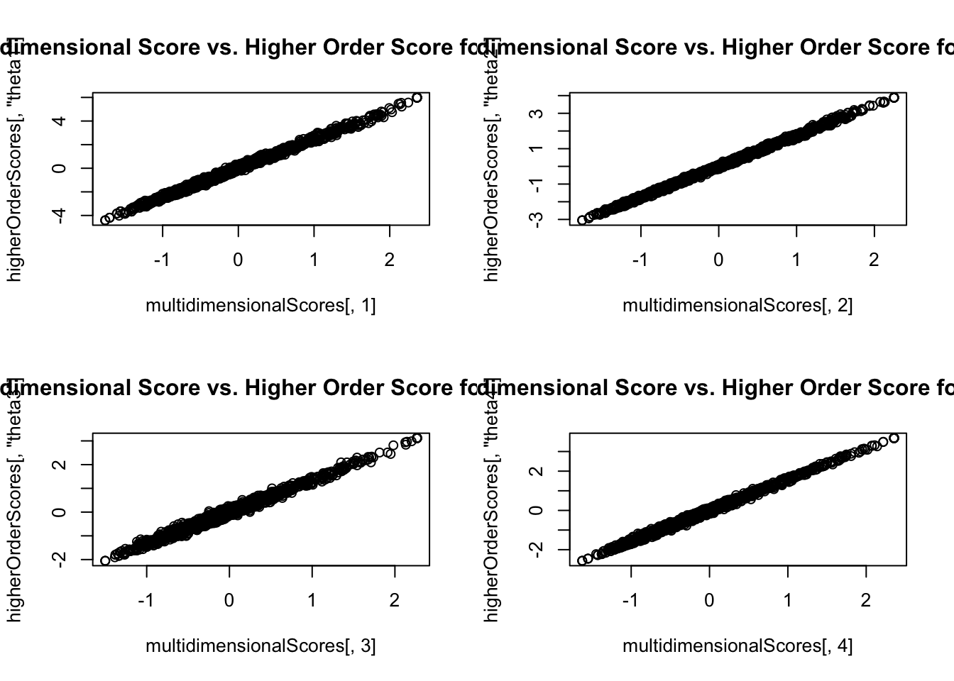
Higher Order Model Score Comparisons: Unidimensional IRT model \(\theta\) vs. Higher Order IRT model \(F\)
= lavPredict (higherOrderModel)plot (x = unidimensionalScores, y = higherOrderScores[, "algebra" ], main = "Unidimensional Score vs. Higher Order Score" )
Higher Order Model Score Comparisons: Standards
par (mfrow = c (2 ,2 ))plot (x = multidimensionalScores[, 1 ], y = higherOrderScores[, "theta1" ],main = "Multidimensional Score vs. Higher Order Score for Theta 1" )plot (x = multidimensionalScores[, 2 ], y = higherOrderScores[, "theta2" ],main = "Multidimensional Score vs. Higher Order Score for Theta 2" )plot (x = multidimensionalScores[, 3 ], y = higherOrderScores[, "theta3" ],main = "Multidimensional Score vs. Higher Order Score for Theta 3" )plot (x = multidimensionalScores[, 4 ], y = higherOrderScores[, "theta4" ],main = "Multidimensional Score vs. Higher Order Score for Theta 4" )
Model Fit Comparison
anova (unidimensionalModel, multidimensionalModel, higherOrderModel)
Scaled Chi-Squared Difference Test (method = "satorra.2000")

lavaan NOTE:
    The "Chisq" column contains standard test statistics, not the
    robust test that should be reported per model. A robust difference
    test is a function of two standard (not robust) statistics.

                       Df AIC BIC  Chisq Chisq diff Df diff Pr(>Chisq)
multidimensionalModel 164         233.93
higherOrderModel      166         252.42     13.261       2    0.00132 **
unidimensionalModel   170         419.00    141.738       4    < 2e-16 ***
---
Signif. codes:  0 '***' 0.001 '**' 0.01 '*' 0.05 '.' 0.1 ' ' 1
So, the higher order model is really what is needed…but, what if it does not fit? * We can use CFA-based tools (modification indices) to help make the model fit better