Markov Chain Monte Carlo Estimation and Stan

SMIP Summer School 2025: Lecture 04

Section Objectives

An Introduction to MCMC
An Introduction to Stan
Both with Linear Models

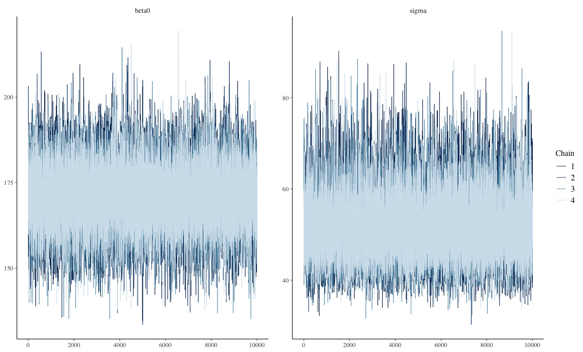
The Markov Chain Timeseries

The Posterior Distribution

Markov Chain Monte Carlo Estimation

Bayesian analysis is all about estimating the posterior distribution

Up until now, we have worked with posterior distributions that are fairly well-known
- Beta-Binomial had a Beta distribution
- In general, likelihood distributions from the exponential family have conjugate priors
  - Conjugate prior: the family of the prior is equivalent to the family of the posterior
Most of the time, however, posterior distributions are not easily obtainable
- No longer able to use properties of the distribution to estimate parameters

Markov Chain Monte Carlo Estimation

It is possible to use an optimization algorithm (e.g., Newton-Raphson or Expectation-Maximization) to find maximum value of posterior distribution
- But, such algorithms may take a very long time for high-dimensional problems
Instead: “sketch” the posterior by sampling from it – then use that sketch to make inferences
- Sampling is done via MCMC

Markov Chain Monte Carlo Estimation

MCMC algorithms iteratively sample from the posterior distribution
- For fairly simplistic models, each iteration has independent samples
- Most models have some layers of dependency included
  - Can slow down sampling from the posterior
There are numerous variations of MCMC algorithms
- Most of these specific algorithms use one of two types of sampling:
  1. Direct sampling from the posterior distribution (i.e. Gibbs sampling)
    - Often used when conjugate priors are specified
  2. Indirect (rejection-based) sampling from the posterior distribution (e.g., Metropolis-Hastings, Hamiltonian Monte Carlo)

MCMC Algorithms

Efficiency is the main reason why there are many different algorithms
- Efficiency in this context: How quickly the algorithm converges and provides adequate coverage (“sketching”) of the posterior distribution
- No one algorithm is uniformly most efficient for all models (here model = likelihood $\times$ prior)
The good news is that many software packages (stan, JAGS, MPlus, especially) don’t make you choose which specific algorithm to use
The bad news is that sometimes your model may take a large amount of time to reach convergence (think days or weeks)
You can also code your own custom algorithm to make things run more smoothly

Commonalities Across MCMC Algorithms

Despite having fairly broad differences regarding how algorithms sample from the posterior distribution, there are quite a few things that are similar across algorithms:
1. A period of the Markov chain where sampling is not directly from the posterior
  - The burnin period (sometimes coupled with other tuning periods and called warm-up)
2. Methods used to assess convergence of the chain to the posterior distribution
  - Often involving the need to use multiple chains with independent and differing starting values

Commonalities Across MCMC Algorithms

Despite having fairly broad differences regarding how algorithms sample from the posterior distribution, there are quite a few things that are similar across algorithms:
1. Summaries of the posterior distribution
Further, rejection-based sampling algorithms often need a tuning period to make the sampling more efficient
- The tuning period comes before the algorithm begins its burnin period

MCMC Demonstration

To demonstrate each type of algorithm, we will use a model for a normal distribution
- We will investigate each, briefly
- We will then switch over to stan to show the syntax and let stan work
- We will conclude by talking about assessing convergence and how to report parameter estimates.

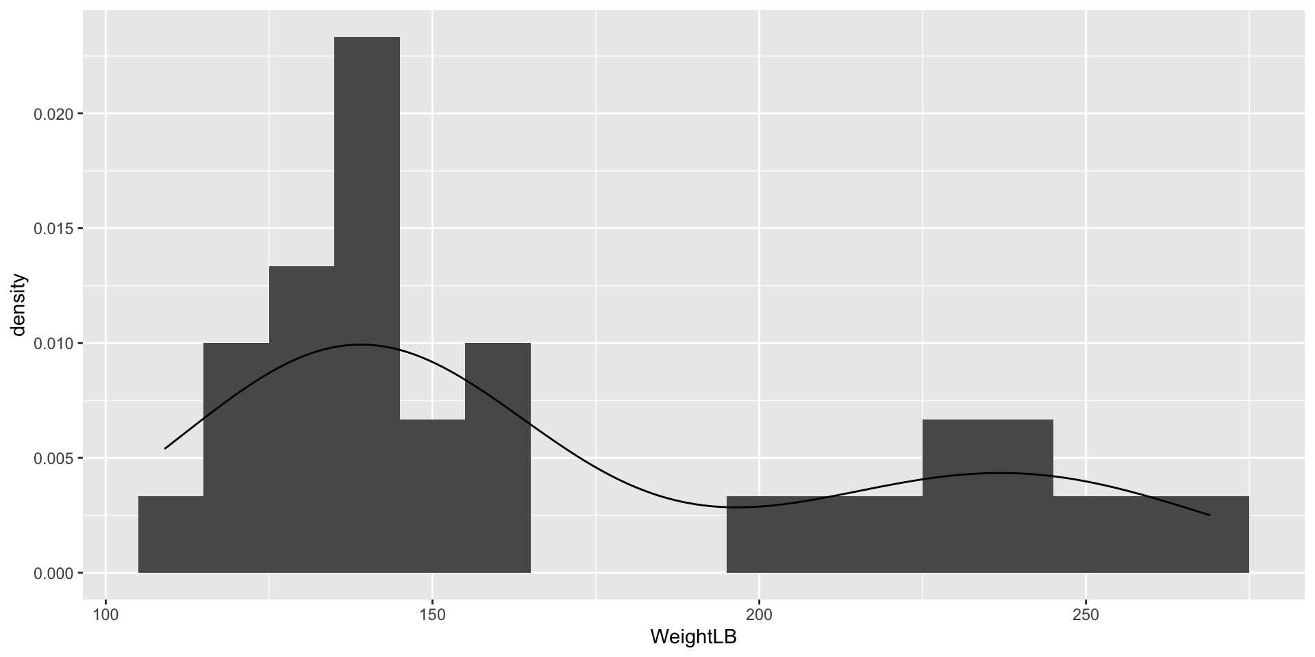
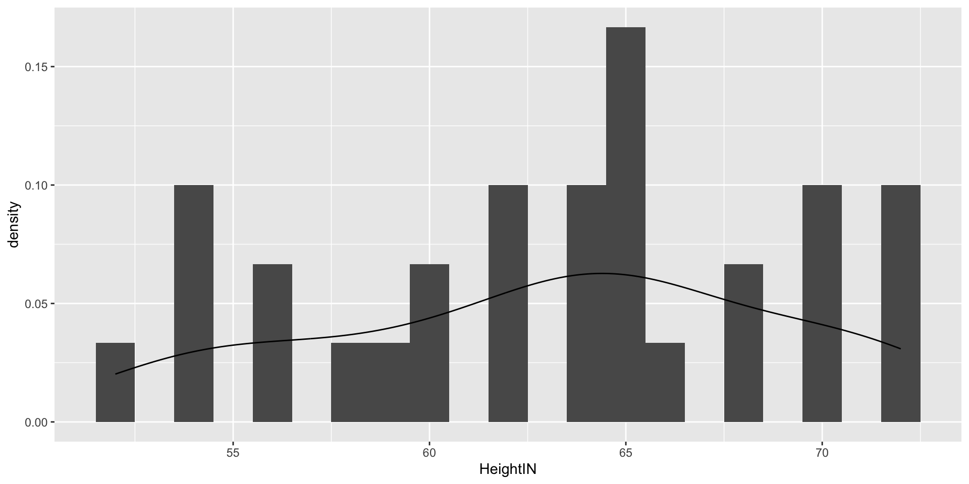
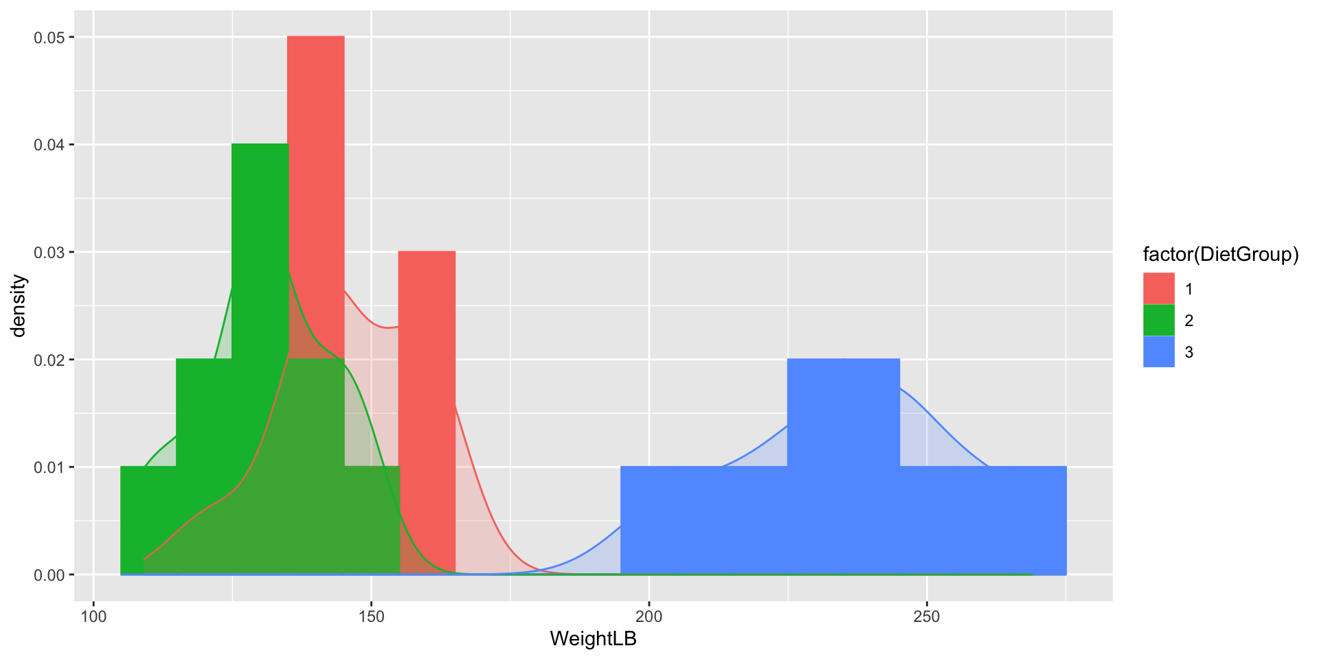
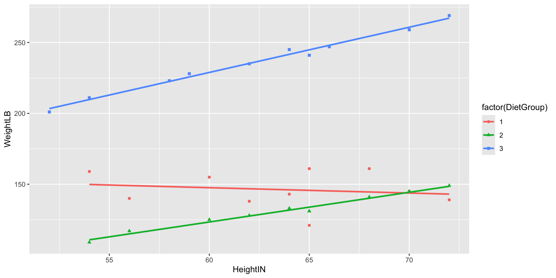
Example Data: Post-Diet Weights

Example Data: https://stats.idre.ucla.edu/spss/library/spss-libraryhow-do-i-handle-interactions-of-continuous-andcategorical-variables/

The file DietData.csv contains data from 30 respondents who participated in a study regarding the effectiveness of three types of diets.
Variables in the data set are:
1. Respondent: Respondent number 1-30
2. DietGroup: A 1, 2, or 3 representing the group to which a respondent was assigned
3. HeightIN: The respondent’s height in inches
4. WeightLB (the Dependent Variable): The respondent’s weight, in pounds, recorded following the study

Example Data: Post-Diet Weights

The research question: Are there differences in final weights between the three diet groups, and, if so, what are the nature of the differences?
But first, let’s look at the data

Visualizing Data: WeightLB Variable

DietData = read.csv(file = "DietData.csv")

ggplot(data = DietData, aes(x = WeightLB)) + 
  geom_histogram(aes(y = ..density..), position = "identity", binwidth = 10) + 
  geom_density(alpha=.2)

Visualizing Data: HeightIN Variable

ggplot(data = DietData, aes(x = HeightIN)) + 
  geom_histogram(aes(y = ..density..), position = "identity", binwidth = 1) + 
  geom_density(alpha=.2)

Visualizing Data: WeightLB by Group

ggplot(data = DietData, aes(x = WeightLB, color = factor(DietGroup), fill = factor(DietGroup))) + 
  geom_histogram(aes(y = ..density..), position = "identity", binwidth = 10) + 
  geom_density(alpha=.2)

Weight by Height by Group

ggplot(data = DietData, aes(x = HeightIN, y = WeightLB, shape = factor(DietGroup), color = factor(DietGroup))) +
  geom_smooth(method = "lm", se = FALSE) + geom_point()

Class Discussion: What Do We Do?

Now, your turn to answer questions:

What type of analysis seems most appropriate for these data?
Is the dependent variable (WeightLB) is appropriate as-is for such analysis or does it need transformed?

Linear Model with Least Squares

Let’s play with models for data…

# center predictors for reasonable numbers
DietData$HeightIN60 = DietData$HeightIN-60

# full analysis model suggested by data:
FullModel = lm(formula = WeightLB ~ 1, data = DietData)

# examining assumptions and leverage of fit
# plot(FullModel)

# looking at ANOVA table
# anova(FullModel)
 
# looking at parameter summary
 summary(FullModel)


Call:
lm(formula = WeightLB ~ 1, data = DietData)

Residuals:
   Min     1Q Median     3Q    Max 
-62.00 -36.75 -24.00  49.00  98.00 

Coefficients:
            Estimate Std. Error t value Pr(>|t|)    
(Intercept)  171.000      9.041   18.91   <2e-16 ***
---
Signif. codes:  0 '***' 0.001 '**' 0.01 '*' 0.05 '.' 0.1 ' ' 1

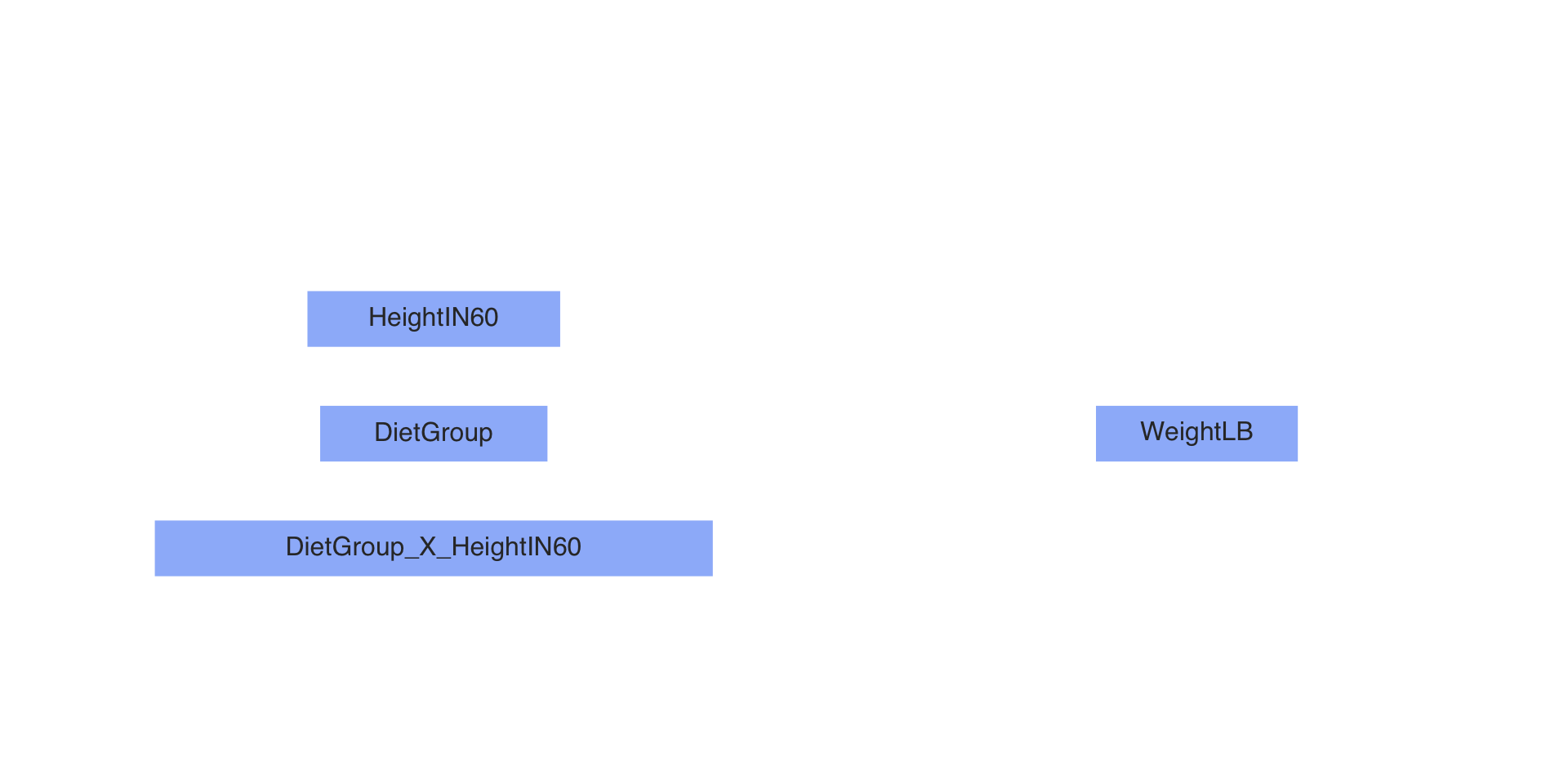
Residual standard error: 49.52 on 29 degrees of freedom

Path Diagram of Our Model

Steps in an MCMC Analysis

Specify model
Specify prior distributions for all model parameters
Build model syntax as needed
Run Markov chains (specify warmup/burnin and sampling period lengths)
Evaluate chain convergence
Interpret/report results

Specify Model

To begin, let’s start with an empty model and build up from there
Let’s examine the linear model we seek to estimate:

\[\text{WeightLB}_p = \beta_0 + e_p,\] Where: $e_p \sim N(0, \sigma^2_e)$

Questions:

What are the variables in this analysis?
What are the parameters in this analysis?

Introduction to Stan

Stan is an MCMC estimation program
- Most recent; has many convenient features
- Actually does severaly methods of estimation (ML, Variational Bayes)
You create a model using Stan’s syntax
- Stan translates your model to a custom-built C++ syntax
- Stan then compiles your model into its own executable program
You then run the program to estimate your model
- If you use R, the interface can be seamless

Stan and RStudio

Stan has its own syntax which can be built in stand-alone text files
- Rstudio will let you create one of these files in the new file menu
- Rstudio also has syntax highlighting in Stan files
  - This is very helpful to learn the syntax
Stan syntax can also be built from R character strings
- Which is helpful when running more than one model per analysis

Stan Syntax

data {
  int<lower=0> N;
  vector[N] y;
}

parameters {
  real beta0;
  real<lower=0> sigma;
}

model {
  beta0 ~ normal(0, 1000); // prior for beta0
  sigma ~ uniform(0, 100000); // prior for sigma
  y ~ normal(beta0, sigma); // model for observed data
}

Each line ends with a semi colon
- Comments are put in with //
Three blocks of syntax needed:
- Data: What Stan expects you will send to it for the analysis (using R lists)
- Parameters: Where you specify what the parameters of the model are
- Model: Where you specify the distributions of the priors and data

Stan Data and Parameter Delcaration

Like many compiled languages, Stan expects you to declare what type of data/parameters you are defining:

int: Integer values (no decimals)
real: Floating point numbers
vector: A one-dimensional set of real valued numbers

Sometimes, additional definitions are provided giving the range of the variable (or restricting the set of starting values):

real<lower=0> sigma;

See: https://mc-stan.org/docs/reference-manual/data-types.html for more information

Stan Data and Prior Distributions

In the model section, you define the distributions needed for the model and the priors
- The left-hand side is either defined in data or parameters
  - y ~ normal(beta0, sigma); // model for observed data
  - sigma ~ uniform(0, 100000); // prior for sigma
- The right-hand side is a distribution included in Stan
  - You can also define your own distributions

See: https://mc-stan.org/docs/functions-reference/index.html for more information

From Stan Syntax to Compilation

# compile model -- this method is for stand-alone stan files (uses cmdstanr)
model00.fromFile = cmdstan_model(stan_file = "model00.stan")

# or this method using the string text in R
model00.fromString = cmdstan_model(stan_file = write_stan_file(stanModel))

Once you have your syntax, next you need to have Stan translate it into C++ and compile an executable
This is where cmdstanr and rstan differ
- cmdstanr wants you to compile first, then run the Markov chain
- rstan conducts compilation (if needed) then runs the Markov chain

Building Data for Stan

# build R list containing data for Stan: Must be named what "data" are listed in analysis
stanData = list(
  N = nrow(DietData),
  y = DietData$WeightLB
)

# snippet of Stan syntax:
stanSyntaxSnippet = "
data {
  int<lower=0> N;
  vector[N] y;
}
"

Stan needs the data you declared in your syntax to be able to run
Within R, we can pass this data to Stan via a list object
The entries in the list should correspond to the data portion of the Stan syntax
- In the above syntax, we told Stan to expect a single integer named N and a vector named y
The R list object is the same for cmdstanr and rstan

Running Markov Chains in `cmdstanr`

# run MCMC chain (sample from posterior)
model00.samples = model00.fromFile$sample(
  data = stanData,
  seed = 1,
  chains = 4,
  parallel_chains = 4,
  iter_warmup = 10000,
  iter_sampling = 10000
)

In cmdstanr, running the chain comes from the $sample() function that is a part of the compiled program object
You must specify:
- The data
- The random number seed
- The number of chains (and parallel chains)
- The number of warmup iterations (more detail shortly)
- The number of sampling iterations

MCMC Process

The MCMC algorithm runs as a series of discrete iterations
- Within each iteration, each parameter of a model has an opportunity to change its value
For each parameter, a new parameter is sampled at random from the current belief of posterior distribution
- The specifics of the sampling process differ by algorithm type (we’ll have a lecture on this later)
In Stan (Hamiltonian Monte Carlo), for a given iteration, a proposed parameter is generated
- The posterior likelihood “values” (more than just density; includes likelihood of proposal) are calculated for the current and proposed values of the parameter
- The proposed values are accepted based on the draw of a uniform number compared to a transition probability
If all models are specified correctly, then regardless of starting location, each chain will converge to the posterior if run long enough
- But, the chains must be checked for convergence when the algorithm stops

Example of Bad Convergence

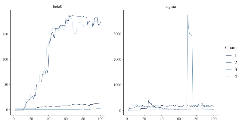
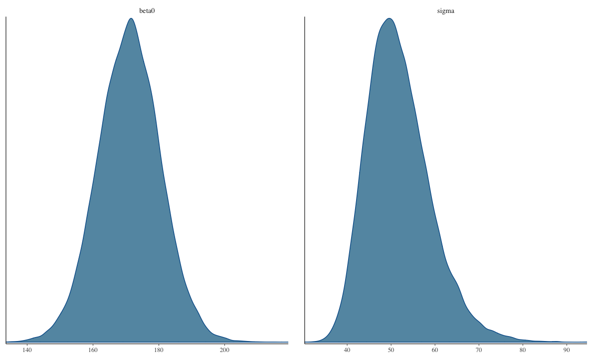
Examining Chain Convergence

Next, we must determine if the chains converged to their posterior distribution
Two most common methods: visual in spection and Gelman-Rubin Potential Scale Reduction Factor (PSRF; quick reference)
Visual inspection
- Want no trends in timeseries – should look like a catapillar
- Shape of posterior density should be mostly smooth
Gelman-Rubin PSRF (denoted with $\hat{R}$)
- For analyses with multiple chains
- Ratio of between-chain variance to within-chain variance
- Should be near 1 (maximum somewhere under 1.05)

Setting MCMC Options

More than one chain should be run: convergence is assessed using multiple chains
- Between-chain variance estimates improve with the number of chains
Warmup/burnin period should be long enough to ensure chains move to center of posterior distribution
- More complex models need more warmup/burnin to converge
Sampling iterations should be long enough to thoroughly sample posterior distribution
- Difficulty to determine ahead of time
- Need smooth densities across bulk of posterior
Often, multiple analyses (with different settings) are needed

The Markov Chain Timeseries

The Posterior Distribution

Assessing Our Chains

model00.samples$summary()

# A tibble: 3 × 10
  variable   mean median    sd   mad     q5    q95  rhat ess_bulk ess_tail
  <chr>     <dbl>  <dbl> <dbl> <dbl>  <dbl>  <dbl> <dbl>    <dbl>    <dbl>
1 lp__     -129.  -128.   1.03 0.737 -131.  -128.   1.00   17204.   21369.
2 beta0     171.   171.   9.52 9.40   155.   187.   1.00   26136.   23619.
3 sigma      51.8   51.0  7.25 6.89    41.5   64.9  1.00   25343.   23597.

The summary function reports the PSRF (rhat)
Here we look at our two parameters: $\beta_0$ and $\sigma$
Both have $\hat{R}=1.00$, so both would be considered converged
lp__ is posterior log likelihood–does not necessarily need examined
ess_ columns show effect sample size for chain (factoring in autocorrelation between correlations)
- More is better

Results Interpretation

At long last, with a set of converged Markov chains, we can now interpret the results
- Here, we disregard which chain samples came from and pool all sampled values to use for results
We use summaries of posterior distributions when describing model parameters
- Typical summary: the posterior mean (called EAP–Expected a Posteriori)
  - The mean of the sampled values in the chain
Important point:
- Posterior means are different than what characterizes the ML estimates
  - Analogous to ML estimates would be the mode of the posterior distribution
- Especially important if looking at non-symmetric posterior distributions
  - Look at posterior for variances

Results Interpretation

To summarize the uncertainty in parameters, we use the posterior standard deviation
- The standard deviation of the sampled values in the chain
- This is the analogous to the standard error from ML
Bayesian credible intervals are formed by taking quantiles of the posterior distribution
- Analogous to confidence intervals
- Interpretation slightly different – the probability the parameter lies within the interval
- 95% credible interval notes that parameter is within interval with 95% confidence
Additionally, highest density posterior intervals can be formed
- The narrowest range for an interval (for unimodal posterior distributions)

Our Results

model00.samples$summary()

# A tibble: 3 × 10
  variable   mean median    sd   mad     q5    q95  rhat ess_bulk ess_tail
  <chr>     <dbl>  <dbl> <dbl> <dbl>  <dbl>  <dbl> <dbl>    <dbl>    <dbl>
1 lp__     -129.  -128.   1.03 0.737 -131.  -128.   1.00   17204.   21369.
2 beta0     171.   171.   9.52 9.40   155.   187.   1.00   26136.   23619.
3 sigma      51.8   51.0  7.25 6.89    41.5   64.9  1.00   25343.   23597.

hdi(model00.samples$draws("beta0"), credMass = .9)

  lower   upper 
154.917 186.013 
attr(,"credMass")
[1] 0.9

hdi(model00.samples$draws("sigma"), credMass = .9)

  lower   upper 
40.3082 63.1433 
attr(,"credMass")
[1] 0.9

The Posterior Distribution

Wrapping Up

This section covered the basics of MCMC estimation with Stan
Next we will use an example to show a full analysis of the item response data problem we started with today
The details today are the same for all MCMC analyses, regardless of which algorithm is used

Markov Chain Monte Carlo Estimation and Stan

Section Objectives

The Markov Chain Timeseries

The Posterior Distribution

Markov Chain Monte Carlo Estimation

Markov Chain Monte Carlo Estimation

Markov Chain Monte Carlo Estimation

MCMC Algorithms

Commonalities Across MCMC Algorithms

Commonalities Across MCMC Algorithms

MCMC Demonstration

Example Data: Post-Diet Weights

Example Data: Post-Diet Weights

Visualizing Data: WeightLB Variable

Visualizing Data: HeightIN Variable

Visualizing Data: WeightLB by Group

Weight by Height by Group

Class Discussion: What Do We Do?

Linear Model with Least Squares

Path Diagram of Our Model

Steps in an MCMC Analysis

Specify Model

Introduction to Stan

Stan and RStudio

Stan Syntax

Stan Data and Parameter Delcaration

Stan Data and Prior Distributions

From Stan Syntax to Compilation

Building Data for Stan

Running Markov Chains in cmdstanr

MCMC Process

Example of Bad Convergence

Examining Chain Convergence

Setting MCMC Options

The Markov Chain Timeseries

The Posterior Distribution

Assessing Our Chains

Results Interpretation

Results Interpretation

Our Results

The Posterior Distribution

Wrapping Up

Running Markov Chains in `cmdstanr`