An Introduction to Regularization Methods

Introduction

Section 1: The Problem with “Best Fit”

Changing Landscape of Data

• Traditional Research: Small \(N\) (participants), Small \(p\) (variables).
  • Focus: Theory-driven hypothesis testing.
• The New Reality: “Wide” Data: Log-trace data, dense surveys, genomic markers.
  • High-Dimensional Prediction: \(p\) is large relative to \(N\).
• The Consequence: Traditional methods like OLS struggle to distinguish signal from noise.

The Status Quo: Ordinary Least Squares (OLS)

• The Gold Standard: OLS is designed for inference in large samples with few predictors.
• The Objective: Unbiased estimates with minimum standard error.
• The Mechanism: Minimizes the Residual Sum of Squares (RSS).
  • It tries to pass a line strictly through the “center” of the data points.

The OLS Trap in High Dimensions

• Capitalizing on Chance: When predictors (\(p\)) are many, OLS finds spurious relationships by chance.
• Overfitting: The model “memorizes” the training data rather than learning the underlying pattern.
• The Symptom: Excellent fit on current data (\(R^2\) is high).
  • Poor performance on new data (Prediction fails).

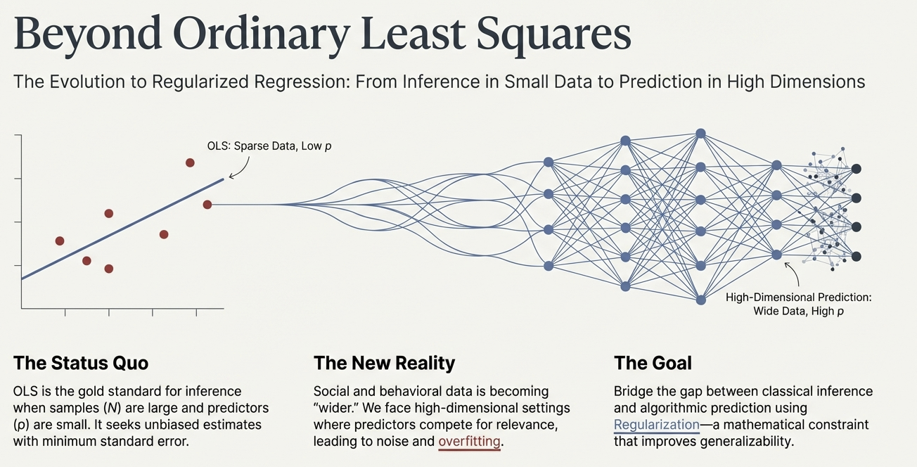
Visualizing the Problem

• Left: OLS works well with sparse data.
• Right: As dimensions expand, the connections become too complex for simple minimization.

As you can see in this graphic, OLS is built for the world on the left. But we are increasingly operating in the world on the right—complex networks of variables. We need a way to navigate this complexity without getting lost in the noise.

The Goal: Generalizability

• Shift in Perspective: Moving from “Is this coefficient significant?” to “Does this model generalize?”.
• The Trade-off: To improve prediction on future data, we must accept some error on current data.
• The Solution: We need a mathematical way to constrain the model—to stop it from chasing noise.

Our goal is no longer just explaining the past; it’s predicting the future. To do this, we have to make a tough trade. We have to sacrifice the “perfect fit” on our training data to build a model that is robust enough to handle new data.

Concept

Section 2: The Solution - Regularization

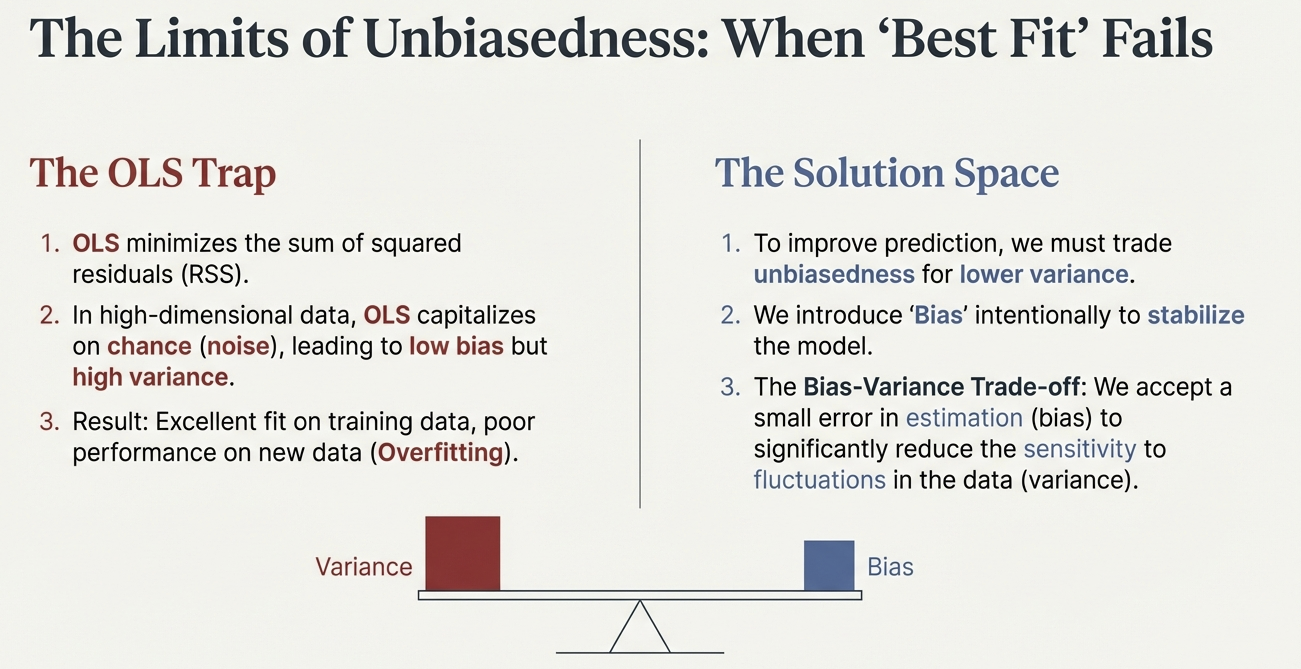
The Bias-Variance Trade-off

• Bias: Error from erroneous assumptions (e.g., missing a relationship).
• Variance: Error from sensitivity to small fluctuations in the training set.
• The Conflict: OLS = Low Bias, High Variance.
  • Regularization = Higher Bias, Low Variance.

This is the fundamental law of machine learning. You cannot have it all. OLS has “High Variance”—if you change your sample slightly, your estimates jump around wildy. Regularization introduces “Bias”—it systematically dampens the estimates—in exchange for “Low Variance.” We prefer the latter because it is stable.

Introducing “Bias” Intentionally

• Why Add Bias? By restricting the model, we stabilize the estimates.
  • We prevent the model from reacting to random noise.
• The Result: A model that is slightly “wrong” on average (biased) but consistently closer to the truth (low variance) across different samples.

It sounds counterintuitive. Why would we want a biased model? Because in a noisy, complex world, a little bit of bias acts like an anchor. It keeps the model from drifting away with every random wave in your data.

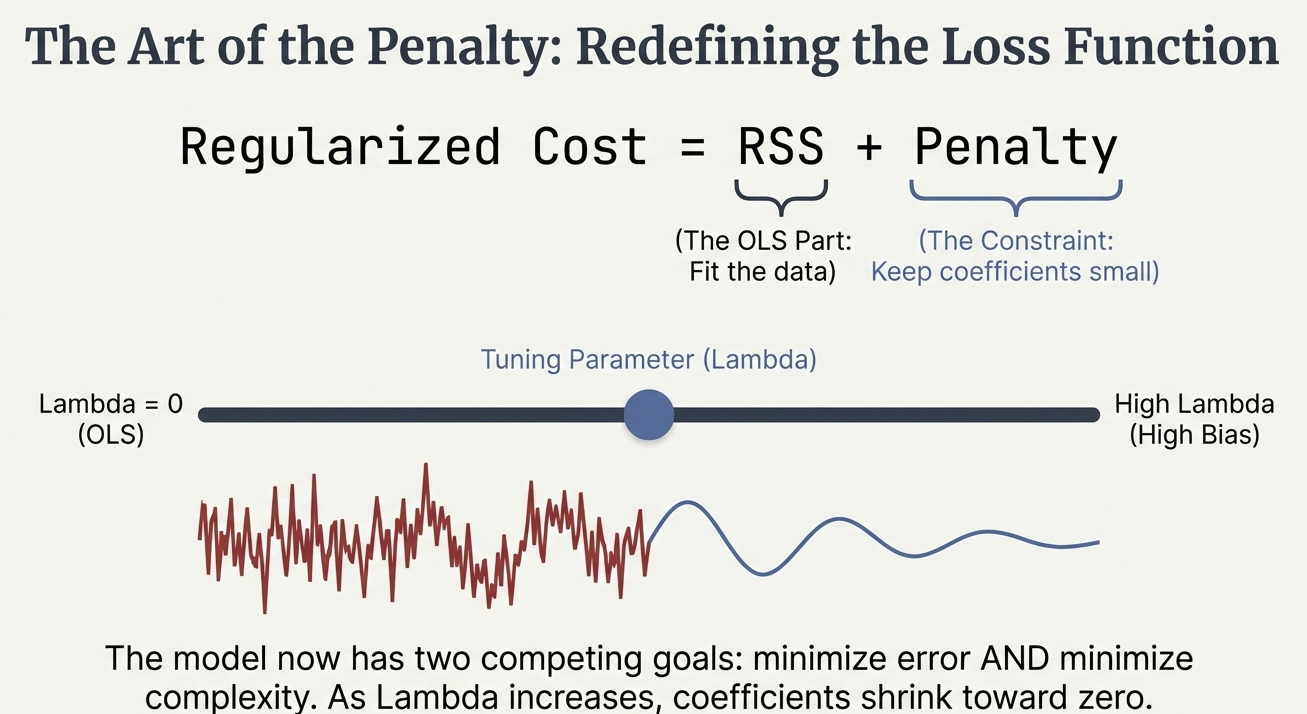
The Math: Redefining the Cost Function

\[\text{Regularized Cost} = \text{[RSS] or [-LL]} + \text{Penalty}\]

• RSS: The standard OLS term (Fit the data).
• Penalty: The constraint term (Keep coefficients small).
• The Mechanism: The model must “pay” a price for every coefficient it estimates.

Here is the math. It’s actually quite simple. We take the standard OLS equation (RSS) and we add a “Penalty” term. Think of this as a tax on complexity. The model wants to minimize error, but now it also wants to minimize this tax.

The Specifics: Linear Models with OLS

The least squares cost function:

\[\text{RSS} = \sum_{p=1}^{N}\left(Y_p - \left(\beta_0 + \sum_{i=1}^{p} \beta_i X_{ip}\right)\right)^2\]

The Specifics: Generalized Linear Models with Maximum Likelihood

The ML likelihood function:

\[\text{LL} = \sum_{p=1}^{N} \log P(Y_p | X_p, \boldsymbol{\beta})\]

• Here, \(P(Y_p | X_p, \boldsymbol{\beta})\) is the PDF of the outcome

The Cost Function

\[\text{Regularized Cost} = \text{[RSS] or [-LL]} + \text{Penalty}\]

• Penalty: A function of the coefficients (\(\beta\)s) that increases as coefficients grow.
• Types of Penalties:
  • Ridge Regression: \(\lambda \sum_{i=1}^{P} \beta_i^2\) (L2 norm)
  • LASSO: \(\lambda \sum_{i=1}^{P} |\beta_i|\) (L1 norm)
  • Elastic Net: \(\lambda \left(\alpha \sum_{i=1}^{P} |\beta_i| + (1-\alpha) \sum_{i=1}^{P} \beta_i^2\right)\)

NOTE: \(\lambda\) and \(\alpha\) are set by the user (and typically ranges of \(\lambda\) are tested)

• The Goal: Minimize the Regularized Cost by choosing optimal \(\beta\)s.

The Tuning Parameter: Lambda (\(\lambda\))

• Lambda (\(\lambda\)): Controls the strength of the penalty.
• \(\lambda = 0\): No penalty. The result is identical to OLS.
• High \(\lambda\): Strong penalty. Coefficients are shrunken heavily toward zero (High Bias).
• The Goal: Find the “Goldilocks” \(\lambda\)—not too simple, not too complex.

This symbol, Lambda, is our tuning knob. If we set it to zero, we get standard regression. As we turn it up, we increase the pressure on the coefficients. If we turn it up too high, we crush everything to zero. Our job is to find the perfect middle ground.

Techniques

Section 3: Ridge Regression

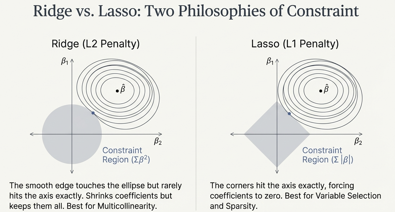
Ridge Regression (\(L_2\) Penalty)

• The Formula: Adds the sum of squared coefficients to the cost function. \[\dots + \lambda \sum \beta^2\]
• Behavior: Shrinks coefficients toward zero but rarely sets them exactly to zero.
  • “Democratic” shrinkage: It reduces the impact of all variables proportionally.

The first type of regularization is Ridge. It penalizes the square of the coefficients. This mathematics results in a “smooth” shrinkage. It makes all the coefficients smaller, but it keeps them all in the model.

Geometric Intuition: The Circle

• Constraint Region: \(\sum \beta^2\) creates a circular constraint.
• The Result: The solution touches the circle but rarely hits the axis (zero) exactly.

Geometrically, Ridge draws a circle around the origin. The regression solution has to stay within this circle. Because the circle is round, the “best fit” point usually hits somewhere along the curve, not strictly on an axis. This means your variables get small, but they don’t disappear.

When to Use Ridge?

• Best Use Case: High Multicollinearity.
  • Example: Multiple survey items measuring the same construct.
• Handling Correlation: OLS would produce unstable estimates with huge standard errors.
  • Ridge shares the credit among correlated predictors, shrinking them together.

Why use Ridge? It is the master of multicollinearity. If you have five survey questions that all correlate highly with each other, OLS will panic and give you wild estimates. Ridge remains calm. It shrinks them all together, sharing the predictive power among them.

Techniques

Section 4: LASSO Regression

LASSO Regression (\(L_1\) Penalty)

• The Formula: Adds the sum of absolute coefficients to the cost function. \[\dots + \lambda \sum |\beta|\]
• Behavior: * Forces coefficients exactly to zero.
  • Performs Variable Selection automatically.

Now we meet the LASSO. This stands for “Least Absolute Shrinkage and Selection Operator.” Instead of squaring the coefficients, we take the absolute value. This small change makes a huge difference.

Geometric Intuition: The Diamond

• Constraint Region: \(\sum |\beta|\) creates a diamond-shaped constraint.
• The Result: The corners of the diamond hit the axes.
  • Hitting an axis means the coefficient for that variable becomes zero.

The absolute value creates a diamond shape with sharp corners. The “best fit” solution is statistically very likely to hit one of these corners. When you hit a corner, that coordinate is zero. This means LASSO literally deletes variables from your model.

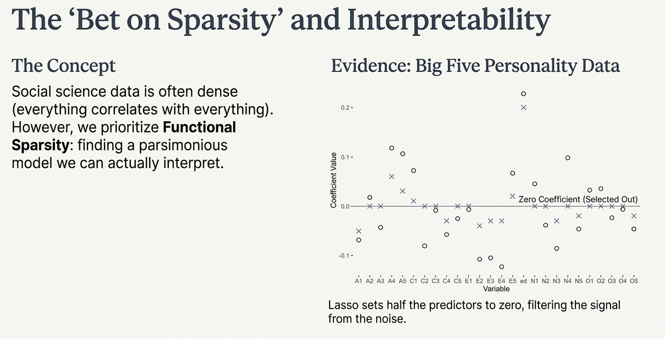
The “Bet on Sparsity”

• Assumption: The underlying truth is “sparse”—only a few variables truly matter.
• Reality in Social Science: Data is often dense (everything correlates with everything).
• Functional Sparsity: We prioritize a parsimonious model we can actually interpret.

LASSO relies on the “Bet on Sparsity”—the idea that only a few predictors are the true drivers. In social science, this is rarely strictly true; everything is connected. However, we often aim for “Functional Sparsity.” We want a simpler model that filters out the noise so we can interpret the strongest signals.

Example: Personality Data

• Context: Predicting an outcome using Big Five personality items (\(p=25\)) + Education.
• Result: LASSO sets nearly half the predictors to zero.
• Benefit: Filters the signal from the noise, leaving a cleaner model.

Here is an example using personality data. We fed the model 26 variables. LASSO (the X marks) set many of them to exactly zero. It decided they weren’t adding enough predictive value to justify the “complexity tax.”

Implementation

Section 5: Practical Application

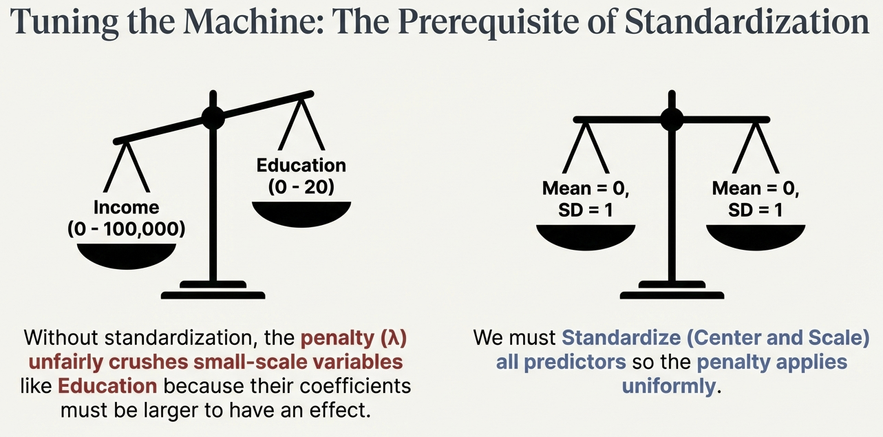
Prerequisite: Standardization

• The Problem: The penalty is uniform. Large-scale variables (Income) have small coefficients; Small-scale variables (GPA) have large coefficients.
• The Consequence: Without scaling, the penalty unfairly crushes variables with small natural scales.
• The Fix: Standardize (Center and Scale) all predictors to Mean=0, SD=1. Categorical variables must be dummy coded before standardization.

Before you run any of this code, you must standardize your data. If you treat Income (0 to 100,000) the same as GPA (0 to 4), the mathematics of the penalty will fail. We standardize everything to Z-scores so the penalty applies to the information, not the units.

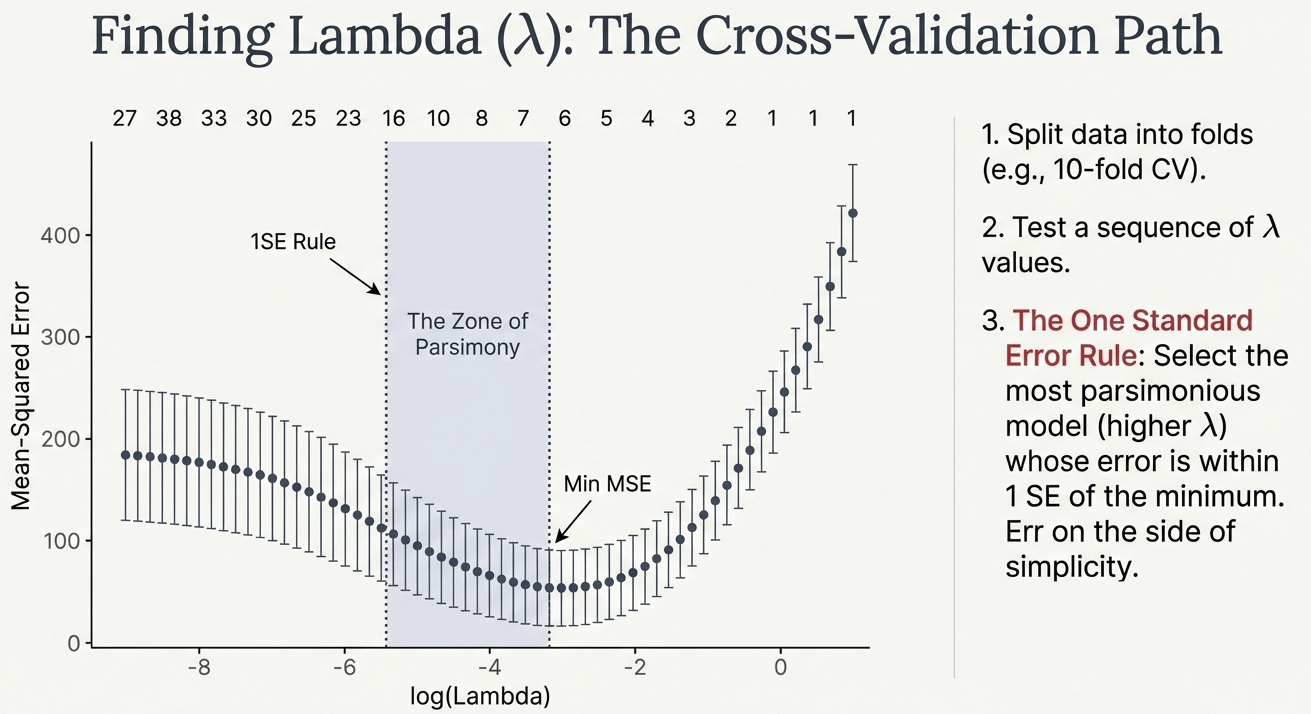
Choosing Lambda: Cross-Validation

• Process:
  1. Split data into folds (e.g., 10-fold CV).
  2. Test a sequence of \(\lambda\) values.
  3. Calculate Mean Squared Error (MSE) for each \(\lambda\).
• Visualization: The “CV Path” shows error changing as complexity changes.

How do we pick Lambda? We let the data decide. We run the model 100 times with different penalty strengths and check the error rate using cross-validation. This plot shows the error curve.

The “One Standard Error Rule”

• Min MSE: The \(\lambda\) value that minimizes error mathematically.
• 1SE Rule: Select the most parsimonious model (higher \(\lambda\)) whose error is within 1 Standard Error of the minimum.
• Why? Err on the side of simplicity. If a simpler model is statistically indistinguishable from the complex one, pick the simple one.

Here is a pro-tip. Don’t just pick the absolute lowest error. We use the “One Standard Error Rule.” We move to the right on the graph—towards more penalty and fewer variables—until the error starts to get significantly worse. This gives us the simplest defensible model.

Advanced Methods

Section 6: Extensions

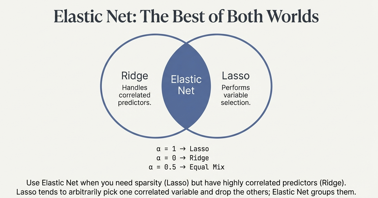
Elastic Net: Best of Both Worlds

• The Limitation of LASSO: If variables are highly correlated, LASSO picks one arbitrarily and drops the rest.
• The Solution: Elastic Net mixes L1 (Lasso) and L2 (Ridge) penalties.
  • \(\alpha\) parameter controls the mix (\(\alpha=0.5\) is equal mix).
• Outcome: Performs selection (Lasso) but keeps correlated groups together (Ridge).

Sometimes you need the best of both worlds. Elastic Net blends Ridge and LASSO. It’s perfect for survey data where you want to drop irrelevant questions but keep grouped questions (scales) intact.

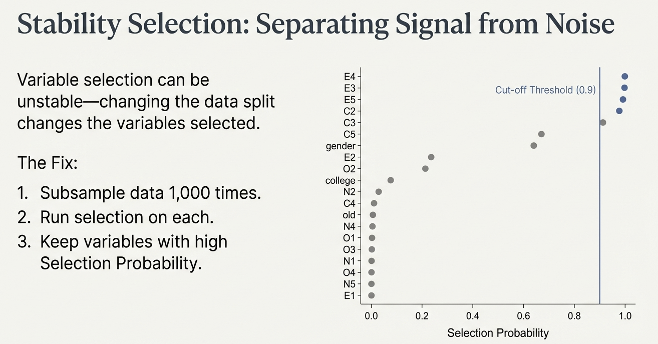
Stability Selection

• The Problem: Variable selection can be unstable. Changing the data split slightly changes which variables are picked.
• The Fix:
  1. Subsample data 1,000 times.
  2. Run selection on each subsample.
  3. Keep variables with high Selection Probability.

If you are worried that your results are a fluke, use Stability Selection. It runs the LASSO 1,000 times on random subsamples. You only keep the variables that survive 90% (or some other threshold) of the time. It separates the robust signal from the noisy flukes.

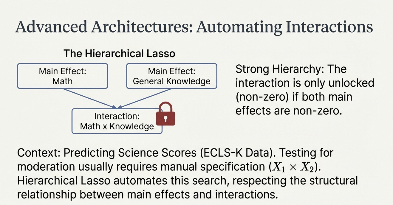
Hierarchical LASSO: Interactions

• Context: Testing moderation (e.g., Treatment \(\times\) Prior Knowledge).
• Challenge: With many predictors, checking all interactions is impossible manually.
• Solution: Hierarchical LASSO automates interaction search.
• Strong Hierarchy: An interaction is only “unlocked” if its main effects are also selected.

For learning scientists, interactions are key. “Does this intervention work for everyone, or just high achievers?” Hierarchical LASSO automates the search for these interactions while enforcing logic—it won’t claim an interaction exists unless the main variables are also important.

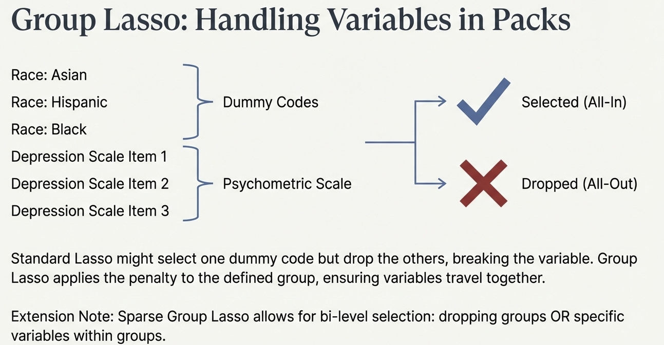
Group LASSO

• Context: Categorical variables (e.g., Race/Ethnicity dummy codes) or psychometric scales.
• Problem: Standard LASSO might drop “Hispanic” but keep “Asian,” breaking the variable structure.
• Solution: Applies penalty to the Group of variables. They are either all included or all dropped.

Finally, if you have categorical variables like Ethnicity, you can’t chop them up. Group LASSO treats the set of dummy codes as a single block. It ensures your demographic controls stay meaningful.

Conclusion: A New Standard

• Embrace Complexity: Regularization allows us to analyze high-dimensional data without being fooled by it.
• Filter Signal from Noise: It provides a principled way to reduce complex data to interpretable models.
• The Future: Moving towards robust, generalizable prediction in the Learning Sciences.

We are entering a new era of data-intensive research. Regularization is not just a fancy trick; it is a necessary adaptation. It allows us to embrace the complexity of learning environments without being fooled by the noise. It helps us build models that don’t just fit the past, but predict the future.