Bayesian Psychometric Model Fit Methods
Today’s Lecture Objectives
- Show how to use PPMC to evaluate absolute model fit in Bayesian psychometric models
- Show how to use LOO and WAIC for relative model fit in Bayesian psychometric models
Example Data: Conspiracy Theories
Today’s example is from a bootstrap resample of 177 undergraduate students at a large state university in the Midwest. The survey was a measure of 10 questions about their beliefs in various conspiracy theories that were being passed around the internet in the early 2010s. Additionally, gender was included in the survey. All items responses were on a 5- point Likert scale with:
- Strongly Disagree
- Disagree
- Neither Agree or Disagree
- Agree
- Strongly Agree
Please note, the purpose of this survey was to study individual beliefs regarding conspiracies. The questions can provoke some strong emotions given the world we live in currently. All questions were approved by university IRB prior to their use.
Our purpose in using this instrument is to provide a context that we all may find relevant as many of these conspiracy theories are still prevalent today.
Conspiracy Theory Questions 1-5
Questions:
- The U.S. invasion of Iraq was not part of a campaign to fight terrorism, but was driven by oil companies and Jews in the U.S. and Israel.
- Certain U.S. government officials planned the attacks of September 11, 2001 because they wanted the United States to go to war in the Middle East.
- President Barack Obama was not really born in the United States and does not have an authentic Hawaiian birth certificate.
- The current financial crisis was secretly orchestrated by a small group of Wall Street bankers to extend the power of the Federal Reserve and further their control of the world’s economy.
- Vapor trails left by aircraft are actually chemical agents deliberately sprayed in a clandestine program directed by government officials.
Conspiracy Theory Questions 6-10
Questions:
- Billionaire George Soros is behind a hidden plot to destabilize the American government, take control of the media, and put the world under his control.
- The U.S. government is mandating the switch to compact fluorescent light bulbs because such lights make people more obedient and easier to control.
- Government officials are covertly Building a 12-lane "NAFTA superhighway" that runs from Mexico to Canada through America’s heartland.
- Government officials purposely developed and spread drugs like crack-cocaine and diseases like AIDS in order to destroy the African American community.
- God sent Hurricane Katrina to punish America for its sins.
Model Setup Today
Today, we will revert back to the graded response model assumptions to discuss how to estimate the latent variable standard deviation
\[P\left(Y_{ic } = c \mid \theta_p \right) = \left\{ \begin{array}{lr} 1-P\left(Y_{i1} \gt 1 \mid \theta_p \right) & \text{if } c=1 \\ P\left(Y_{i{c-1}} \gt c-1 \mid \theta_p \right) - P\left(Y_{i{c}} \gt c \mid \theta_p \right) & \text{if } 1<c<C_i \\ P\left(Y_{i{C_i -1} } \gt C_i-1 \mid \theta_p \right) & \text{if } c=C_i \\ \end{array} \right.\]
Where:
\[ P\left(Y_{i{c}} > c \mid \theta \right) = \frac{\exp(-\tau_{ic}+\lambda_i\theta_p)}{1+\exp(-\tau_{ic}+\lambda_i\theta_p)}\]
With:
- \(C_i-1\) Ordered thresholds: \(\tau_1 < \tau_2 < \ldots < \tau_{C_i-1}\)
We can convert thresholds to intercepts by multiplying by negative one: \(\mu_c = -\tau_c\)
Model Comparisons: One vs. Two Dimensions
We will fit two models to the data:
- A unidimensional model (see Lecture 4d here)
- A two-dimensionsal model (see Lecture 4e here)
We know from previous lectures that the two-dimensional model had a correlation very close to one
- Such a high correlation made it seem implausible there were two dimensions
Posterior Predictive Model Checking for Absolute Fit in Bayesian Psychometric Models
Psychometric Model PPMC
Psychometric models can use posterior predictive model checking (PPMC) to assess how well they fit the data in an absolute sense
- Each iteration of the chain, each item is simulated using model parameter values from that iteration
- Summary statistics are used to evaluate model fit
- Univariate measures (each item, separately):
- Item mean
- Item \(\chi^2\) (comparing observed data with each simulated data set)
- Not very useful unless:
- Parameters have “obscenely” informative priors
- There are cross-item constraints on some parameters (such as all loadings are equal)
- Bivariate measures (each pair of items)
- For binary data: Tetrachoric correlations
- For polytomous data: Polychoric correlations (but difficult to estimate with small samples), pearson correlations
- For other types of data: Pearson correlations
- Univariate measures (each item, separately):
Problems with PPMC
Problems with PPMC include
- No uniform standard for which statistics to use
- Tetrachoric correlations? Pearson correlations?
- No uniform standard by which data should fit, absolutely
- Jihong Zhang has some work on this topic, though:
- Paper in Structural Equation Modeling
- Dissertation on PPMC with M2 statistics (working on publishing)
- Jihong Zhang has some work on this topic, though:
- No way to determine if a model is overparameterized (too complicated)
- Fit only improves to a limit
Implementing PPMC in Stan (one \(\theta\))
Notes:
- Generated quantities block is where to implement PPMC
- Each type of distribution also has a random number generator
- Here,
ordered_logistic_rnggoes withordered_logistic
- Here,
- Each may have some issue in types of inputs (had to go person-by-person in this block)
- Rather than have Stan calculate statistics, I will do so in R
Implementing PPMC in Stan (two \(\theta\)s)
Notes:
- Very similar to one dimension–just using the syntax from the model block within the
ordered_logistic_rngfunction
PPMC Processing
Stan generated a lot of data–but now we must take it from the format of Stan and process it:
# setting up PPMC
simData = modelOrderedLogit_samples$draws(variables = "simY", format = "draws_matrix")
colnames(simData)
dim(simData)


# set up object for storing each iteration's PPMC data
nPairs = choose(10, 2)
pairNames = NULL
for (col in 1:(nItems-1)){
  for (row in (col+1):nItems){
    pairNames = c(pairNames, paste0("item", row, "_item", col))
  }
}
PPMC Calculating in R
PPMCsamples = list()

PPMCsamples$correlation = NULL
PPMCsamples$mean = NULL

# loop over each posterior sample's simulated data

for (sample in 1:nrow(simData)){

  # create data frame that has observations (rows) by items (columns)
  sampleData = data.frame(matrix(data = NA, nrow = nObs, ncol = nItems))

  for (item in 1:nItems){
    itemColumns = colnames(simData)[grep(pattern = paste0("simY\\[", item, "\\,"), x = colnames(simData))]
    sampleData[,item] = t(simData[sample, itemColumns])
  }
  # with data frame created, apply functions of the data:

  # calculate item means
  PPMCsamples$mean = rbind(PPMCsamples$mean, apply(X = sampleData, MARGIN = 2, FUN = mean))

  # calculate pearson correlations
  temp=cor(sampleData)
  PPMCsamples$correlation = rbind(PPMCsamples$correlation, temp[lower.tri(temp)])


}
PPMC Results Tabulation in R (Mean)
# next, build distributions for each type of statistic
meanSummary = NULL

# for means
for (item in 1:nItems){

  tempDist = ecdf(PPMCsamples$mean[,item])
  ppmcMean = mean(PPMCsamples$mean[,item])
  observedMean = mean(conspiracyItems[,item])
  meanSummary = rbind(
    meanSummary,
    data.frame(
      item = paste0("Item", item),
      ppmcMean = ppmcMean,
      observedMean = observedMean,
      residual = observedMean - ppmcMean,
      observedMeanPCT = tempDist(observedMean)
    )
  )

}
PPMC Results Tabulation in R (Correlation)
# for pearson correlations
corrSummary = NULL
# for means
for (column in 1:ncol(PPMCsamples$correlation)){
# get item numbers from items
items = unlist(strsplit(x = colnames(PPMCsamples$correlation)[column], split = "_"))
item1num = as.numeric(substr(x = items[1], start = 5, stop = nchar(items[1])))
item2num = as.numeric(substr(x = items[2], start = 5, stop = nchar(items[2])))
tempDist = ecdf(PPMCsamples$correlation[,column])
ppmcCorr = mean(PPMCsamples$correlation[,column])
observedCorr = cor(conspiracyItems[,c(item1num, item2num)])[1,2]
pct = tempDist(observedCorr)
if (pct > .975 | pct < .025){
inTail = TRUE
} else {
inTail = FALSE
}
corrSummary = rbind(
corrSummary,
data.frame(
item1 = paste0("Item", item1num),
item2 = paste0("Item", item2num),
ppmcCorr = ppmcCorr,
observedCorr = observedCorr,
residual = observedCorr - ppmcCorr,
observedCorrPCT = pct,
inTail = inTail
)
)
}
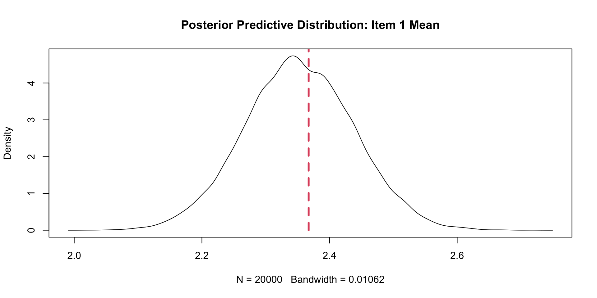
View(corrSummary)PPMC Mean Results: Example Item (One \(\theta\))
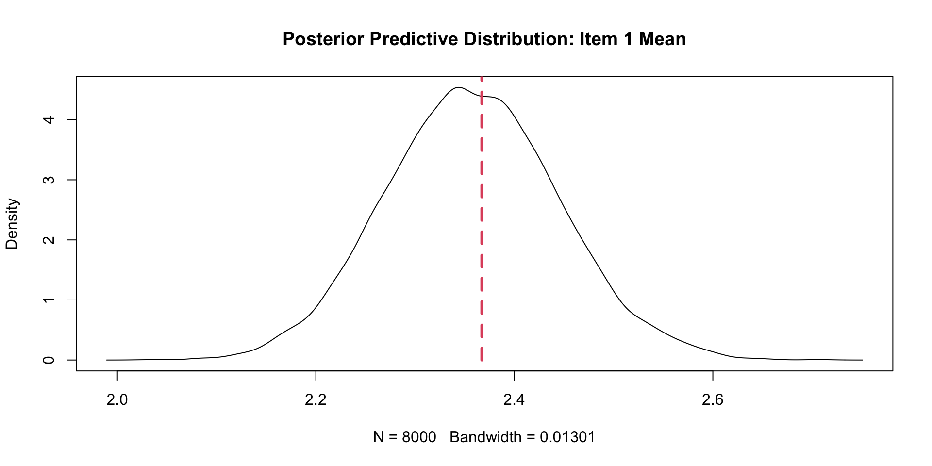
PPMC Mean Results: Example Item (Two \(\theta\)s)
PPMC Mean Results
One \(\theta\)
     item ppmcMean observedMean     residual observedMeanPCT
1   Item1 2.352560     2.367232  0.014671186         0.58340
2   Item2 1.958342     1.954802 -0.003539831         0.47495
3   Item3 1.862719     1.875706  0.012987571         0.58610
4   Item4 2.008068     2.011299  0.003231638         0.53915
5   Item5 1.978207     1.983051  0.004843503         0.53005
6   Item6 1.880974     1.892655  0.011681356         0.61725
7   Item7 1.748335     1.723164 -0.025171469         0.37290
8   Item8 1.840580     1.841808  0.001228249         0.51550
9   Item9 1.825317     1.807910 -0.017407062         0.43230
10 Item10 1.535198     1.519774 -0.015424294         0.45225
Two \(\theta\)s
item ppmcMean observedMean residual observedMeanPCT
1 Item1 2.357626 2.367232 0.0096059322 0.559500
2 Item2 1.969614 1.954802 -0.0148114407 0.418500
3 Item3 1.874785 1.875706 0.0009216102 0.528000
4 Item4 2.016655 2.011299 -0.0053552260 0.493000
5 Item5 1.988220 1.983051 -0.0051687853 0.465375
6 Item6 1.895842 1.892655 -0.0031864407 0.500375
7 Item7 1.758951 1.723164 -0.0357874294 0.326125
8 Item8 1.853244 1.841808 -0.0114357345 0.424500
9 Item9 1.835992 1.807910 -0.0280819209 0.373625
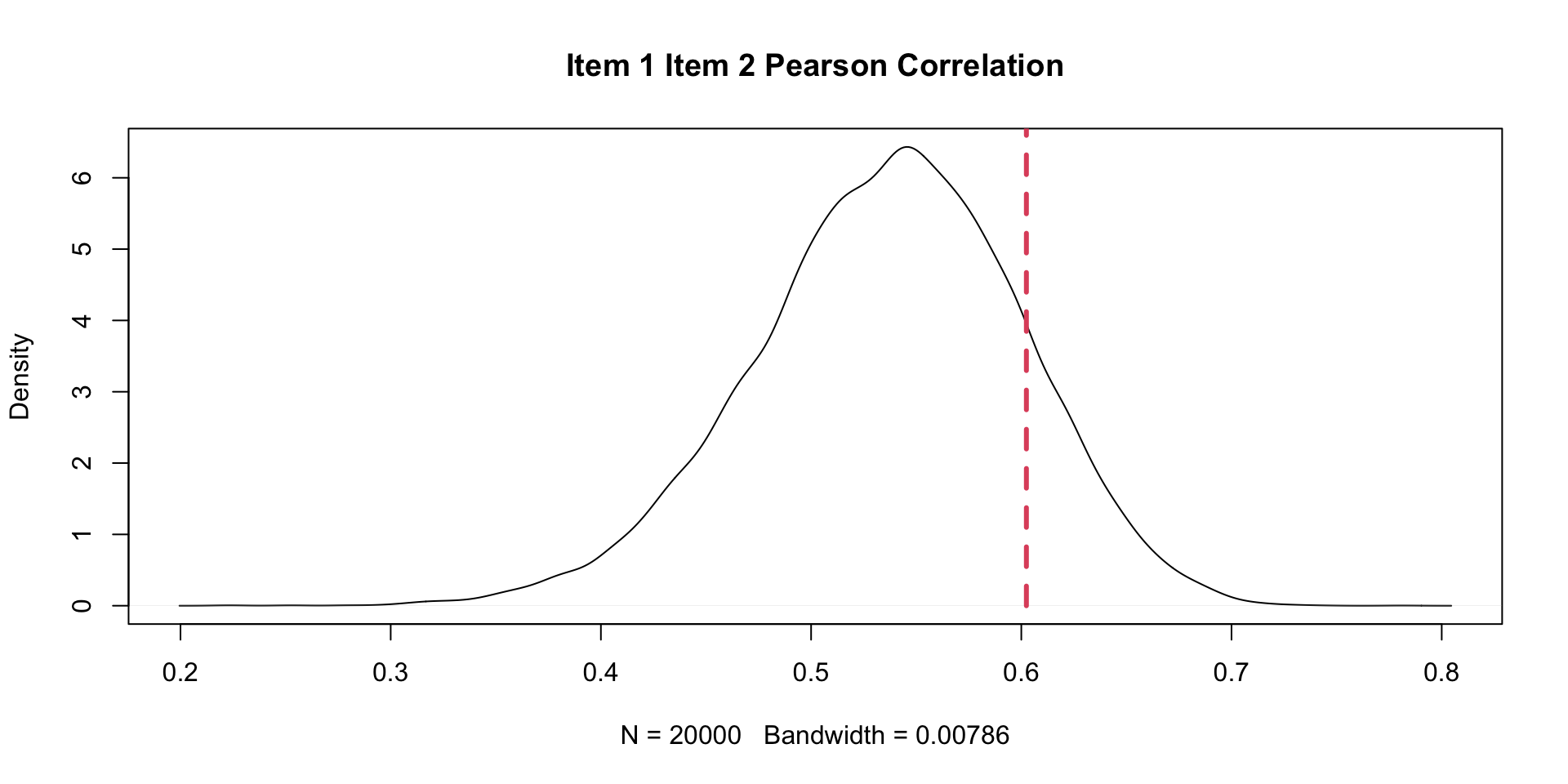
10 Item10 1.553063 1.519774 -0.0332888418 0.376125PPMC Correlation Results: Example Item Pair (One \(\theta\))
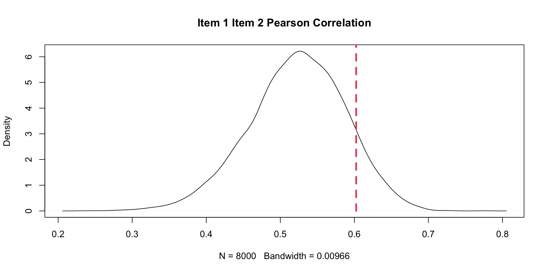
PPMC Correlation Results: Example Item Pair (Two \(\theta\)s)
PPMC Correlation Results
    item1 item2 observedCorr ppmcCorr.x   residual.x observedCorrPCT.x inTail.x
1  Item10 Item1    0.2568334  0.4131131 -0.156279686           0.01655     TRUE
2  Item10 Item2    0.4121264  0.4917030 -0.079576626           0.14375    FALSE
3  Item10 Item3    0.5670156  0.4522000  0.114815615           0.93835    FALSE
4  Item10 Item4    0.4516124  0.4890239 -0.037411565           0.28790    FALSE
5  Item10 Item5    0.5822203  0.5567640  0.025456304           0.62005    FALSE
6  Item10 Item6    0.5092003  0.5501939 -0.040993565           0.25890    FALSE
7  Item10 Item7    0.4420205  0.4992130 -0.057192487           0.22315    FALSE
8  Item10 Item8    0.5457127  0.5434373  0.002275470           0.48760    FALSE
9  Item10 Item9    0.4244916  0.4940797 -0.069588089           0.18525    FALSE
10  Item2 Item1    0.6024186  0.5357365  0.066682114           0.85585    FALSE
11  Item3 Item1    0.3473072  0.4931202 -0.145812943           0.01745     TRUE
12  Item3 Item2    0.5176819  0.5569093 -0.039227387           0.26420    FALSE
13  Item4 Item1    0.5700901  0.5439901  0.026099947           0.64290    FALSE
14  Item4 Item2    0.5815808  0.6090530 -0.027472228           0.30375    FALSE
15  Item4 Item3    0.4973987  0.5615192 -0.064120482           0.15380    FALSE
16  Item5 Item1    0.5526073  0.6008370 -0.048229709           0.19820    FALSE
17  Item5 Item2    0.6512768  0.6835423 -0.032265485           0.25645    FALSE
18  Item5 Item3    0.5942163  0.6288536 -0.034637387           0.26495    FALSE
19  Item5 Item4    0.6267160  0.6877014 -0.060985378           0.11495    FALSE
20  Item6 Item1    0.5435771  0.5996223 -0.056045208           0.16460    FALSE
21  Item6 Item2    0.6835282  0.6802492  0.003279028           0.49990    FALSE
22  Item6 Item3    0.6601292  0.6276426  0.032486611           0.68855    FALSE
23  Item6 Item4    0.6251455  0.6853371 -0.060191526           0.11720    FALSE
24  Item6 Item5    0.7366890  0.7696183 -0.032929309           0.18445    FALSE
25  Item7 Item1    0.4084389  0.5196236 -0.111184764           0.04695    FALSE
26  Item7 Item2    0.4721628  0.5988845 -0.126721659           0.02785    FALSE
27  Item7 Item3    0.6193269  0.5520486  0.067278349           0.83690    FALSE
28  Item7 Item4    0.4676834  0.6002957 -0.132612336           0.02010     TRUE
29  Item7 Item5    0.6204485  0.6779012 -0.057452711           0.14370    FALSE
30  Item7 Item6    0.6870303  0.6740562  0.012974158           0.57020    FALSE
31  Item8 Item1    0.5425166  0.5990322 -0.056515657           0.16485    FALSE
32  Item8 Item2    0.6317705  0.6774062 -0.045635698           0.17995    FALSE
33  Item8 Item3    0.6182736  0.6266373 -0.008363667           0.42020    FALSE
34  Item8 Item4    0.6373299  0.6835823 -0.046252488           0.17135    FALSE
35  Item8 Item5    0.7641703  0.7672351 -0.003064875           0.44260    FALSE
36  Item8 Item6    0.7557355  0.7697220 -0.013986520           0.33825    FALSE
37  Item8 Item7    0.6611475  0.6720005 -0.010853042           0.39345    FALSE
38  Item9 Item1    0.4420860  0.5114050 -0.069318985           0.14180    FALSE
39  Item9 Item2    0.5998366  0.5909206  0.008915976           0.53460    FALSE
40  Item9 Item3    0.3912734  0.5436816 -0.152408206           0.01670     TRUE
41  Item9 Item4    0.6108052  0.5917868  0.019018393           0.60460    FALSE
42  Item9 Item5    0.7119365  0.6693743  0.042562230           0.76780    FALSE
43  Item9 Item6    0.5849045  0.6643001 -0.079395555           0.07880    FALSE
44  Item9 Item7    0.5653926  0.5905836 -0.025191060           0.33045    FALSE
45  Item9 Item8    0.6068774  0.6608282 -0.053950800           0.15570    FALSE
   ppmcCorr.y   residual.y observedCorrPCT.y inTail.y
1   0.4062453 -0.149411838          0.021375     TRUE
2   0.4741188 -0.061992441          0.208000    FALSE
3   0.4396909  0.127324771          0.954625    FALSE
4   0.4789946 -0.027382240          0.337625    FALSE
5   0.5336977  0.048522599          0.736750    FALSE
6   0.5316488 -0.022448494          0.350250    FALSE
7   0.4725387 -0.030518156          0.338000    FALSE
8   0.5166837  0.029028985          0.646500    FALSE
9   0.4749625 -0.050470922          0.258750    FALSE
10  0.5225588  0.079859795          0.897625    FALSE
11  0.4845009 -0.137193683          0.025250    FALSE
12  0.5407355 -0.023053619          0.348375    FALSE
13  0.5350439  0.035046168          0.693625    FALSE
14  0.5943265 -0.012745647          0.396500    FALSE
15  0.5518686 -0.054469852          0.197875    FALSE
16  0.5823830 -0.029775722          0.296250    FALSE
17  0.6655675 -0.014290652          0.375000    FALSE
18  0.6060217 -0.011805479          0.396875    FALSE
19  0.6653200 -0.038603963          0.219375    FALSE
20  0.5827271 -0.039150054          0.242750    FALSE
21  0.6534385  0.030089655          0.701875    FALSE
22  0.6077661  0.052363175          0.802875    FALSE
23  0.6669047 -0.041759184          0.201375    FALSE
24  0.7328579  0.003831089          0.509500    FALSE
25  0.5004824 -0.092043558          0.087625    FALSE
26  0.5787187 -0.106555900          0.051250    FALSE
27  0.5271264  0.092200572          0.912500    FALSE
28  0.5763177 -0.108634364          0.048625    FALSE
29  0.6497289 -0.029280447          0.293375    FALSE
30  0.6379156  0.049114716          0.802500    FALSE
31  0.5730756 -0.030559026          0.295375    FALSE
32  0.6518795 -0.020108970          0.331750    FALSE
33  0.5950893  0.023184359          0.626625    FALSE
34  0.6538394 -0.016509531          0.355250    FALSE
35  0.7305302  0.033640008          0.771125    FALSE
36  0.7215552  0.034180334          0.770375    FALSE
37  0.6364697  0.024677809          0.647000    FALSE
38  0.5001129 -0.058026879          0.189375    FALSE
39  0.5797217  0.020114922          0.602250    FALSE
40  0.5287277 -0.137454306          0.028625    FALSE
41  0.5774416  0.033363627          0.688875    FALSE
42  0.6522837  0.059652847          0.848125    FALSE
43  0.6383018 -0.053397216          0.170875    FALSE
44  0.5700175 -0.004624969          0.456375    FALSE
45  0.6362707 -0.029393327          0.285125    FALSE
Count of Items in Misfitting Pairs
One \(\theta\)
badItems
 Item1  Item3 Item10  Item4  Item7  Item9
     2      2      1      1      1      1
Two \(\theta\)s
badItems2
 Item1 Item10
     1      1
Plotting Misfitting Items (One \(\theta\))
Relative Model Fit in Bayesian Psychometric Models
Relative Model Fit in Bayesian Psychometric Models
As with other Bayesian models, we can use WAIC and LOO to compare the model fit of two Bayesian models
- Of note: There is some debate as to whether or not we should marginalize across the latent variables
- We won’t do that here as that would involve a numeric integral
- What is needed: The conditional log likelihood for each observation at each step of the chain
- Here, we have to sum the log likelihood across all items
- There are built-in functions in Stan to do this
Implementing ELPD in Stan (one \(\theta\))
generated quantities{

  // for LOO/WAIC:
  vector[nObs] personLike = rep_vector(0.0, nObs);

  for (item in 1:nItems){
    for (obs in 1:nObs){
      // calculate conditional data likelihood for LOO/WAIC
      personLike[obs] = personLike[obs] + ordered_logistic_lpmf(Y[item, obs] | lambda[item]*theta[obs], thr[item]);
    }
  }
}
Notes:
ordered_logistic_lpmfneeds the observed data to work (first argument)vector[nObs] personLike = rep_vector(0.0, nObs);is needed to set the values to zero at each iteration
Implementing ELPD in Stan (two \(\theta\)s)
generated quantities{

  // for LOO/WAIC:
  vector[nObs] personLike = rep_vector(0.0, nObs);

  for (item in 1:nItems){
    for (obs in 1:nObs){
      // calculate conditional data likelihood for LOO/WAIC
      personLike[obs] = personLike[obs] + ordered_logistic_lpmf(Y[item, obs] | thetaMatrix[obs,]*lambdaMatrix[item,1:nFactors]', thr[item]);
    }
  }
}
Notes:
ordered_logistic_lpmfneeds the observed data to work (first argument)vector[nObs] personLike = rep_vector(0.0, nObs);is needed to set the values to zero at each iteration
Comparing WAIC Values
Computed from 20000 by 177 log-likelihood matrix

          Estimate    SE
elpd_waic  -1482.6  70.4
p_waic       137.7   5.1
waic        2965.2 140.8

173 (97.7%) p_waic estimates greater than 0.4. We recommend trying loo instead.
Computed from 8000 by 177 log-likelihood matrix

          Estimate    SE
elpd_waic  -1490.6  68.0
p_waic       142.6   4.6
waic        2981.1 136.1

174 (98.3%) p_waic estimates greater than 0.4. We recommend trying loo instead.
Smaller is better, so the unidimensional model wins (but very high SE for both)
Comparing LOO Values
Computed from 20000 by 177 log-likelihood matrix

         Estimate    SE
elpd_loo  -1542.0  71.0
p_loo       197.1   5.8
looic      3084.0 141.9
------
Monte Carlo SE of elpd_loo is NA.

Pareto k diagnostic values:
                         Count Pct.    Min. n_eff
(-Inf, 0.5]   (good)       0    0.0%   <NA>
 (0.5, 0.7]   (ok)         4    2.3%   426
   (0.7, 1]   (bad)      156   88.1%   31
   (1, Inf)   (very bad)  17    9.6%   10
See help('pareto-k-diagnostic') for details.
Computed from 8000 by 177 log-likelihood matrix

         Estimate    SE
elpd_loo  -1541.3  68.1
p_loo       193.2   5.1
looic      3082.5 136.2
------
Monte Carlo SE of elpd_loo is NA.

Pareto k diagnostic values:
                         Count Pct.    Min. n_eff
(-Inf, 0.5]   (good)       1    0.6%   743
 (0.5, 0.7]   (ok)        19   10.7%   42
   (0.7, 1]   (bad)      135   76.3%   4
   (1, Inf)   (very bad)  22   12.4%   4
See help('pareto-k-diagnostic') for details.
LOO seems to (slightly) prefer the two-dimensional model (but by warnings about bad PSIS)
Comparing LOO Values
loo_compare(list(unidimensional = modelOrderedLogit_samples$loo(variables = "personLike"),
                 twodimensional = modelOrderedLogit2D_samples$loo(variables = "personLike")))
elpd_diff se_diff
twodimensional 0.0 0.0
unidimensional -0.7 4.9 Again, both models are very close in fit
Wrapping Up
Wrapping Up
Model fit is complicated for psychometric models
- Bayesian model fit methods are even more complicated than non-Bayesian methods
- Open area for research!
Thank you for a great semester